hyperbolic%20analog

SearchAdvancedHelp

(0.002 seconds)

11—20 of 269 matching pages

11: 4.41 Sums

§4.41 Sums

►For sums of hyperbolic functions see Gradshteyn and Ryzhik (2000, Chapter 1), Hansen (1975, §43), Prudnikov et al. (1986a, §5.3), and Zucker (1979).

12: 4.34 Derivatives and Differential Equations

§4.34 Derivatives and Differential Equations

… ►

4.34.4 $$\frac{d}{dz}\mathrm{csch}z=-\mathrm{csch}z\coth z,$$

ⓘ

Symbols:

$\frac{df}{dx}$: derivative of $f$ with respect to $x$ , $\mathrm{csch}z$: hyperbolic cosecant function, $\coth z$: hyperbolic cotangent function and $z$: complex variable

A&S Ref:

4.5.74

Permalink:

http://dlmf.nist.gov/4.34.E4

Encodings:

pMML, png, TeX

See also:

Annotations for §4.34 and Ch.4

►

4.34.5 $$\frac{d}{dz}\mathrm{sech}z=-\mathrm{sech}z\tanh z,$$

ⓘ

Symbols:

$\frac{df}{dx}$: derivative of $f$ with respect to $x$ , $\mathrm{sech}z$: hyperbolic secant function, $\tanh z$: hyperbolic tangent function and $z$: complex variable

A&S Ref:

4.5.75

Permalink:

http://dlmf.nist.gov/4.34.E5

Encodings:

pMML, png, TeX

See also:

Annotations for §4.34 and Ch.4

… ►With $a\ne 0$, the general solutions of the differential equations … ►

4.34.11 $$w=A\cosh \left(az\right)+B\sinh \left(az\right),$$

ⓘ

Symbols:

$\cosh z$: hyperbolic cosine function, $\sinh z$: hyperbolic sine function, $a$: real or complex constant, $z$: complex variable, $w$: solution, $A$: arbitrary constant and $B$: arbitrary constant

Permalink:

http://dlmf.nist.gov/4.34.E11

Encodings:

pMML, png, TeX

See also:

Annotations for §4.34 and Ch.4

…

13: Bibliography M

… ►

A $q$-analog of the ${}_5{}^{}F_4^{}(1)$ summation theorem for hypergeometric series well-poised in $\mathrm{𝑆𝑈}(n)$ . Adv. in Math. 57 (1), pp. 14–33.

ⓘ

External Links:

ISSN 0001-8708, Document, MathReview (Mourad E. H. Ismail), ZentralBlatt

Referenced by:

§17.15.

Encodings:

BibTeX

… ►

A $q$-analog of hypergeometric series well-poised in $\mathrm{𝑆𝑈}(n)$ and invariant $G$-functions. Adv. in Math. 58 (1), pp. 1–60.

ⓘ

External Links:

ISSN 0001-8708, Document, MathReview (Robert A. Gustafson), ZentralBlatt

Referenced by:

§17.15.

Encodings:

BibTeX

►

A $q$-analog of the Gauss summation theorem for hypergeometric series in $U(n)$ . Adv. in Math. 72 (1), pp. 59–131.

ⓘ

External Links:

ISSN 0001-8708, Document, MathReview (David M. Bressoud), ZentralBlatt

Referenced by:

§17.15.

Encodings:

BibTeX

►

A $q$-analog of a Whipple’s transformation for hypergeometric series in $U(n)$ . Adv. Math. 108 (1), pp. 1–76.

ⓘ

External Links:

ISSN 0001-8708, Document, MathReview, ZentralBlatt

Referenced by:

§17.15.

Encodings:

BibTeX

… ►

The $q$-analogue of the Laguerre polynomials. J. Math. Anal. Appl. 81 (1), pp. 20–47.

ⓘ

External Links:

ISSN 0022-247X, Document, MathReview (R. A. Askey), ZentralBlatt

Referenced by:

§18.27(v).

Encodings:

BibTeX

…

14: 20.11 Generalizations and Analogs

§20.11 Generalizations and Analogs

… ►It is a discrete analog of theta functions. If both $m,n$ are positive, then $G(m,n)$ allows inversion of its arguments as a modular transformation (compare (23.15.3) and (23.15.4)): …This is the discrete analog of the Poisson identity (§1.8(iv)). …

15: 4.40 Integrals

§4.40 Integrals

… ►

§4.40(ii) Indefinite Integrals

… ►

§4.40(iii) Definite Integrals

… ►

§4.40(iv) Inverse Hyperbolic Functions

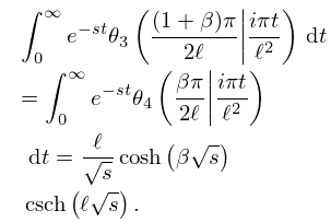
… ►Extensive compendia of indefinite and definite integrals of hyperbolic functions include Apelblat (1983, pp. 96–109), Bierens de Haan (1939), Gröbner and Hofreiter (1949, pp. 139–160), Gröbner and Hofreiter (1950, pp. 160–167), Gradshteyn and Ryzhik (2000, Chapters 2–4), and Prudnikov et al. (1986a, §§1.4, 1.8, 2.4, 2.8).

16: 20.10 Integrals

… ►

20.10.4 $${\int }_0^{\mathrm{\infty }}{\mathrm{e}}^{-st}{\theta }_1\left(\frac{\beta \pi }{2\mathrm{\ell }}\right|\frac{\mathrm{i}\pi t}{{\mathrm{\ell }}^2})dt={\int }_0^{\mathrm{\infty }}{\mathrm{e}}^{-st}{\theta }_2\left(\frac{(1+\beta )\pi }{2\mathrm{\ell }}\right|\frac{\mathrm{i}\pi t}{{\mathrm{\ell }}^2})dt=-\frac{\mathrm{\ell }}{\sqrt{s}}\sinh \left(\beta \sqrt{s}\right)\mathrm{sech}\left(\mathrm{\ell }\sqrt{s}\right),$$

ⓘ

Symbols:

${\theta }_j\left(z\right|\tau )$: theta function, $\pi$: the ratio of the circumference of a circle to its diameter, $dx$: differential of $x$ , $\mathrm{e}$: base of natural logarithm, $\mathrm{sech}z$: hyperbolic secant function, $\sinh z$: hyperbolic sine function, $\mathrm{i}$: imaginary unit, $\int$: integral, $s$: parameter, $\beta$: parameter and $\mathrm{\ell }$: parameter

Permalink:

http://dlmf.nist.gov/20.10.E4

Encodings:

pMML, png, TeX

See also:

Annotations for §20.10(ii), §20.10 and Ch.20

►

20.10.5 $${\int }_0^{\mathrm{\infty }}{\mathrm{e}}^{-st}{\theta }_3\left(\frac{(1+\beta )\pi }{2\mathrm{\ell }}\right|\frac{\mathrm{i}\pi t}{{\mathrm{\ell }}^2})dt={\int }_0^{\mathrm{\infty }}{\mathrm{e}}^{-st}{\theta }_4\left(\frac{\beta \pi }{2\mathrm{\ell }}\right|\frac{\mathrm{i}\pi t}{{\mathrm{\ell }}^2})dt=\frac{\mathrm{\ell }}{\sqrt{s}}\cosh \left(\beta \sqrt{s}\right)\mathrm{csch}\left(\mathrm{\ell }\sqrt{s}\right).$$

ⓘ

Symbols:

${\theta }_j\left(z\right|\tau )$: theta function, $\pi$: the ratio of the circumference of a circle to its diameter, $dx$: differential of $x$ , $\mathrm{e}$: base of natural logarithm, $\mathrm{csch}z$: hyperbolic cosecant function, $\cosh z$: hyperbolic cosine function, $\mathrm{i}$: imaginary unit, $\int$: integral, $s$: parameter, $\beta$: parameter and $\mathrm{\ell }$: parameter

Permalink:

http://dlmf.nist.gov/20.10.E5

Encodings:

pMML, png, TeX

See also:

Annotations for §20.10(ii), §20.10 and Ch.20

…

17: 4.36 Infinite Products and Partial Fractions

§4.36 Infinite Products and Partial Fractions

►

4.36.1 $$\sinh z=z\prod _{n=1}^{\mathrm{\infty }}\left(1+\frac{z^2}{n^2{\pi }^2}\right),$$

ⓘ

Symbols:

$\pi$: the ratio of the circumference of a circle to its diameter, $\sinh z$: hyperbolic sine function, $n$: integer and $z$: complex variable

A&S Ref:

4.5.68

Permalink:

http://dlmf.nist.gov/4.36.E1

Encodings:

pMML, png, TeX

See also:

Annotations for §4.36 and Ch.4

►

4.36.2 $$\cosh z=\prod _{n=1}^{\mathrm{\infty }}\left(1+\frac{4z^2}{{(2n-1)}^2{\pi }^2}\right).$$

ⓘ

Symbols:

$\pi$: the ratio of the circumference of a circle to its diameter, $\cosh z$: hyperbolic cosine function, $n$: integer and $z$: complex variable

A&S Ref:

4.5.69

Permalink:

http://dlmf.nist.gov/4.36.E2

Encodings:

pMML, png, TeX

See also:

Annotations for §4.36 and Ch.4

… ►

4.36.3 $$\coth z=\frac{1}{z}+2z\sum _{n=1}^{\mathrm{\infty }}\frac{1}{z^2+n^2{\pi }^2},$$

ⓘ

Symbols:

$\pi$: the ratio of the circumference of a circle to its diameter, $\coth z$: hyperbolic cotangent function, $n$: integer and $z$: complex variable

Permalink:

http://dlmf.nist.gov/4.36.E3

Encodings:

pMML, png, TeX

See also:

Annotations for §4.36 and Ch.4

►

4.36.4 $${\mathrm{csch}}^{2}z=\sum _{n=-\mathrm{\infty }}^{\mathrm{\infty }}\frac{1}{{(z-n\pi \mathrm{i})}^2},$$

ⓘ

Symbols:

$\pi$: the ratio of the circumference of a circle to its diameter, $\mathrm{csch}z$: hyperbolic cosecant function, $\mathrm{i}$: imaginary unit, $n$: integer and $z$: complex variable

Permalink:

http://dlmf.nist.gov/4.36.E4

Encodings:

pMML, png, TeX

See also:

Annotations for §4.36 and Ch.4

…

18: 4.33 Maclaurin Series and Laurent Series

§4.33 Maclaurin Series and Laurent Series

►

4.33.1 $$\sinh z=z+\frac{z^3}{3!}+\frac{z^5}{5!}+\mathrm{\cdots },$$

ⓘ

Symbols:

$!$: factorial (as in $n!$), $\sinh z$: hyperbolic sine function and $z$: complex variable

A&S Ref:

4.5.62

Permalink:

http://dlmf.nist.gov/4.33.E1

Encodings:

pMML, png, TeX

See also:

Annotations for §4.33 and Ch.4

►

4.33.2 $$\cosh z=1+\frac{z^2}{2!}+\frac{z^4}{4!}+\mathrm{\cdots }.$$

ⓘ

Symbols:

$!$: factorial (as in $n!$), $\cosh z$: hyperbolic cosine function and $z$: complex variable

A&S Ref:

4.5.63

Permalink:

http://dlmf.nist.gov/4.33.E2

Encodings:

pMML, png, TeX

See also:

Annotations for §4.33 and Ch.4

►

4.33.3 $$\tanh z=z-\frac{z^3}{3}+\frac{2}{15}{z}^5-\frac{17}{315}{z}^7+\mathrm{\cdots }+\frac{2^{2n}(2^{2n}-1)B_{2n}}{(2n)!}{z}^{2n-1}+\mathrm{\cdots },$$ .

ⓘ

Symbols:

$B_n$: Bernoulli numbers, $\pi$: the ratio of the circumference of a circle to its diameter, $!$: factorial (as in $n!$), $\tanh z$: hyperbolic tangent function, $n$: integer and $z$: complex variable

A&S Ref:

4.5.64

Permalink:

http://dlmf.nist.gov/4.33.E3

Encodings:

pMML, png, TeX

See also:

Annotations for §4.33 and Ch.4

…

19: 4.47 Approximations

§4.47 Approximations

►

§4.47(i) Chebyshev-Series Expansions

►Clenshaw (1962) and Luke (1975, Chapter 3) give 20D coefficients for $\ln$, $\exp$, $\sin$, $\cos$, $\tan$, $\cot$, $\arcsin$, $\arctan$, $\mathrm{arcsinh}$. … ►Hart et al. (1968) give $\ln$, $\exp$, $\sin$, $\cos$, $\tan$, $\cot$, $\arcsin$, $\arccos$, $\arctan$, $\sinh$, $\cosh$, $\tanh$, $\mathrm{arcsinh}$, $\mathrm{arccosh}$. … ►Luke (1975, Chapter 3) supplies real and complex approximations for $\ln$, $\exp$, $\sin$, $\cos$, $\tan$, $\arctan$, $\mathrm{arcsinh}$. …

20: 36.3 Visualizations of Canonical Integrals

… ►

…

Figure 36.3.9: Modulus of hyperbolic umbilic canonical integral function $|{\mathrm{\Psi }}^{(\mathrm{H})}\left(x,y,0\right)|$.

►

…

Figure 36.3.10: Modulus of hyperbolic umbilic canonical integral function $|{\mathrm{\Psi }}^{(\mathrm{H})}\left(x,y,1\right)|$.

►

…

Figure 36.3.11: Modulus of hyperbolic umbilic canonical integral function $|{\mathrm{\Psi }}^{(\mathrm{H})}\left(x,y,2\right)|$.

►

…

Figure 36.3.12: Modulus of hyperbolic umbilic canonical integral function $|{\mathrm{\Psi }}^{(\mathrm{H})}\left(x,y,3\right)|$.

… ►

…

Figure 36.3.18: Phase of hyperbolic umbilic canonical integral $\mathrm{ph}{\mathrm{\Psi }}^{(\mathrm{H})}\left(x,y,0\right)$.

…