epsilon function

SearchAdvancedHelp

(0.004 seconds)

11—20 of 63 matching pages

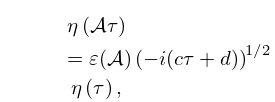
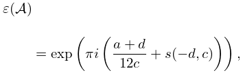
11: 23.18 Modular Transformations

… ►

23.18.5 $$\eta \left(𝒜\tau \right)=\epsilon (𝒜){\left(-\mathrm{i}(c\tau +d)\right)}^{1/2}\eta \left(\tau \right),$$

ⓘ

Symbols:

$\eta \left(\tau \right)$: Dedekind’s eta function (or Dedekind modular function), $\mathrm{i}$: imaginary unit, $\tau$: complex variable, $𝒜$: bilinear transformation, $c$: integer, $d$: integer and $\epsilon (𝒜)$: function

Permalink:

http://dlmf.nist.gov/23.18.E5

Encodings:

pMML, png, TeX

See also:

Annotations for §23.18, §23.18 and Ch.23

►where the square root has its principal value and ►

23.18.6 $$\epsilon (𝒜)=\exp \left(\pi \mathrm{i}\left(\frac{a+d}{12c}+s(-d,c)\right)\right),$$

ⓘ

Symbols:

$\pi$: the ratio of the circumference of a circle to its diameter, $\exp z$: exponential function, $\mathrm{i}$: imaginary unit, $𝒜$: bilinear transformation, $a$: integer, $c$: integer, $d$: integer and $\epsilon (𝒜)$: function

Permalink:

http://dlmf.nist.gov/23.18.E6

Encodings:

pMML, png, TeX

See also:

Annotations for §23.18, §23.18 and Ch.23

…

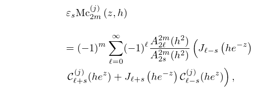
12: 33.16 Connection Formulas

… ►

§33.16(i) $F_{\mathrm{\ell }}$ and $G_{\mathrm{\ell }}$ in Terms of $f$ and $h$

… ►

§33.16(ii) $f$ and $h$ in Terms of $F_{\mathrm{\ell }}$ and $G_{\mathrm{\ell }}$ when $ϵ>0$

… ►

§33.16(iii) $f$ and $h$ in Terms of $W_{\kappa ,\mu }\left(z\right)$ when

… ►

§33.16(iv) $s$ and $c$ in Terms of $F_{\mathrm{\ell }}$ and $G_{\mathrm{\ell }}$ when $ϵ>0$

… ►

§33.16(v) $s$ and $c$ in Terms of $W_{\kappa ,\mu }\left(z\right)$ when

…

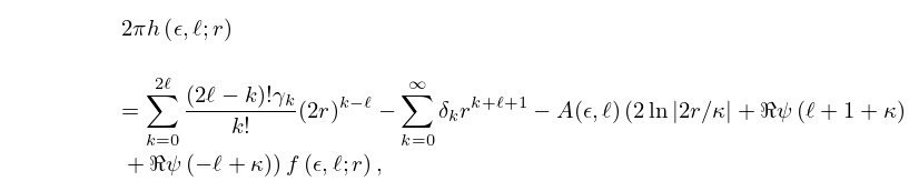
13: 33.19 Power-Series Expansions in $r$

§33.19 Power-Series Expansions in $r$

►

33.19.1 $$f(ϵ,\mathrm{\ell };r)=r^{\mathrm{\ell }+1}\sum _{k=0}^{\mathrm{\infty }}{\alpha }_k{r}^k,$$

ⓘ

Symbols:

$f(ϵ,\mathrm{\ell };r)$: regular Coulomb function, $k$: nonnegative integer, $\mathrm{\ell }$: nonnegative integer, $r$: real variable, $ϵ$: real parameter and ${\alpha }_k$: term

Referenced by:

§33.18, §33.19

Permalink:

http://dlmf.nist.gov/33.19.E1

Encodings:

pMML, png, TeX

See also:

Annotations for §33.19 and Ch.33

… ►

33.19.3 $$2\pi h(ϵ,\mathrm{\ell };r)=\sum _{k=0}^{2\mathrm{\ell }}\frac{(2\mathrm{\ell }-k)!{\gamma }_k}{k!}{(2r)}^{k-\mathrm{\ell }}-\sum _{k=0}^{\mathrm{\infty }}{\delta }_k{r}^{k+\mathrm{\ell }+1}-A(ϵ,\mathrm{\ell })\left(2\ln |2r/\kappa |+\mathrm{\Re }\psi \left(\mathrm{\ell }+1+\kappa \right)+\mathrm{\Re }\psi \left(-\mathrm{\ell }+\kappa \right)\right)f(ϵ,\mathrm{\ell };r),$$ $r\ne 0$.

ⓘ

Symbols:

$f(ϵ,\mathrm{\ell };r)$: regular Coulomb function, $h(ϵ,\mathrm{\ell };r)$: irregular Coulomb function, $\pi$: the ratio of the circumference of a circle to its diameter, $\psi \left(z\right)$: psi (or digamma) function, $!$: factorial (as in $n!$), $\ln z$: principal branch of logarithm function, $\mathrm{\Re }$: real part, $k$: nonnegative integer, $\mathrm{\ell }$: nonnegative integer, $r$: real variable, $ϵ$: real parameter, $\kappa$: quantity, $A(ϵ,\mathrm{\ell })$: function, ${\gamma }_k$: term and ${\delta }_k$: term

Referenced by:

§33.19

Permalink:

http://dlmf.nist.gov/33.19.E3

Encodings:

pMML, png, TeX

See also:

Annotations for §33.19 and Ch.33

… ►

33.19.6 $$k(k+2\mathrm{\ell }+1){\delta }_k+2{\delta }_{k-1}+ϵ{\delta }_{k-2}+2(2k+2\mathrm{\ell }+1)A(ϵ,\mathrm{\ell }){\alpha }_k=0,$$ $k=2,3,\mathrm{\dots }$,

ⓘ

Symbols:

$k$: nonnegative integer, $\mathrm{\ell }$: nonnegative integer, $ϵ$: real parameter, $A(ϵ,\mathrm{\ell })$: function, ${\alpha }_k$: term and ${\delta }_k$: term

Permalink:

http://dlmf.nist.gov/33.19.E6

Encodings:

pMML, png, TeX

See also:

Annotations for §33.19 and Ch.33

…

14: 33.24 Tables

§33.24 Tables

… ►

Curtis (1964a) tabulates $P_{\mathrm{\ell }}(ϵ,r)$, $Q_{\mathrm{\ell }}(ϵ,r)$ (§33.1), and related functions for $\mathrm{\ell }=0,1,2$ and $ϵ=-2(.2)2$, with $x=0(.1)4$ for and $x=0(.1)10$ for $ϵ\ge 0$; 6D.

…

15: 33.1 Special Notation

… ►The main functions treated in this chapter are first the Coulomb radial functions $F_{\mathrm{\ell }}(\eta ,\rho )$, $G_{\mathrm{\ell }}(\eta ,\rho )$, $H_{\mathrm{\ell }}^{\pm }(\eta ,\rho )$ (Sommerfeld (1928)), which are used in the case of repulsive Coulomb interactions, and secondly the functions $f(ϵ,\mathrm{\ell };r)$, $h(ϵ,\mathrm{\ell };r)$, $s(ϵ,\mathrm{\ell };r)$, $c(ϵ,\mathrm{\ell };r)$ (Seaton (1982, 2002a)), which are used in the case of attractive Coulomb interactions. … ►

$f^{(0)}(ϵ,\mathrm{\ell };r)=f(ϵ,\mathrm{\ell };r)$, $f(ϵ,\mathrm{\ell };r)=s(ϵ,\mathrm{\ell };r)$, $g(ϵ,\mathrm{\ell };r)=c(ϵ,\mathrm{\ell };r)$.

16: 28.24 Expansions in Series of Cross-Products of Bessel Functions or Modified Bessel Functions

… ►

28.24.2 $${\epsilon }_s{\mathrm{Mc}}_{2m}^{(j)}(z,h)={(-1)}^m\sum _{\mathrm{\ell }=0}^{\mathrm{\infty }}{(-1)}^{\mathrm{\ell }}\frac{A_{2\mathrm{\ell }}^{2m}(h^2)}{A_{2s}^{2m}(h^2)}\left(J_{\mathrm{\ell }-s}\left(h{\mathrm{e}}^{-z}\right){𝒞}_{\mathrm{\ell }+s}^{(j)}(h{\mathrm{e}}^z)+J_{\mathrm{\ell }+s}\left(h{\mathrm{e}}^{-z}\right){𝒞}_{\mathrm{\ell }-s}^{(j)}(h{\mathrm{e}}^z)\right),$$

ⓘ

Symbols:

$J_{\nu }\left(z\right)$: Bessel function of the first kind, $\mathrm{e}$: base of natural logarithm, ${\mathrm{Mc}}_n^{(j)}(z,h)$: radial Mathieu function, $m$: integer, $h$: parameter, $j$: integer, $z$: complex variable, ${𝒞}_{\mu }^{(j)}$: cylinder functions, ${\epsilon }_s$: constants and $A_m(q)$: Fourier coefficient

A&S Ref:

20.6.7

Permalink:

http://dlmf.nist.gov/28.24.E2

Encodings:

pMML, png, TeX

See also:

Annotations for §28.24 and Ch.28

… ►

28.24.6 $${\epsilon }_s{\mathrm{Ie}}_{2m}(z,h)={(-1)}^s\sum _{\mathrm{\ell }=0}^{\mathrm{\infty }}{(-1)}^{\mathrm{\ell }}\frac{A_{2\mathrm{\ell }}^{2m}(h^2)}{A_{2s}^{2m}(h^2)}\left(I_{\mathrm{\ell }-s}\left(h{\mathrm{e}}^{-z}\right)I_{\mathrm{\ell }+s}\left(h{\mathrm{e}}^z\right)+I_{\mathrm{\ell }+s}\left(h{\mathrm{e}}^{-z}\right)I_{\mathrm{\ell }-s}\left(h{\mathrm{e}}^z\right)\right),$$

ⓘ

Symbols:

$\mathrm{e}$: base of natural logarithm, $I_{\nu }\left(z\right)$: modified Bessel function of the first kind, ${\mathrm{Ie}}_n(z,h)$: modified Mathieu function, $m$: integer, $h$: parameter, $z$: complex variable, ${\epsilon }_s$: constants and $A_m(q)$: Fourier coefficient

A&S Ref:

20.8.8

Permalink:

http://dlmf.nist.gov/28.24.E6

Encodings:

pMML, png, TeX

See also:

Annotations for §28.24 and Ch.28

… ►

28.24.10 $${\epsilon }_s{\mathrm{Ke}}_{2m}(z,h)=\sum _{\mathrm{\ell }=0}^{\mathrm{\infty }}\frac{A_{2\mathrm{\ell }}^{2m}(h^2)}{A_{2s}^{2m}(h^2)}\left(I_{\mathrm{\ell }-s}\left(h{\mathrm{e}}^{-z}\right)K_{\mathrm{\ell }+s}\left(h{\mathrm{e}}^z\right)+I_{\mathrm{\ell }+s}\left(h{\mathrm{e}}^{-z}\right)K_{\mathrm{\ell }-s}\left(h{\mathrm{e}}^z\right)\right),$$

ⓘ

Symbols:

$\mathrm{e}$: base of natural logarithm, $I_{\nu }\left(z\right)$: modified Bessel function of the first kind, $K_{\nu }\left(z\right)$: modified Bessel function of the second kind, ${\mathrm{Ke}}_n(z,h)$: modified Mathieu function, $m$: integer, $h$: parameter, $z$: complex variable, ${\epsilon }_s$: constants and $A_m(q)$: Fourier coefficient

A&S Ref:

20.8.9

Permalink:

http://dlmf.nist.gov/28.24.E10

Encodings:

pMML, png, TeX

See also:

Annotations for §28.24 and Ch.28

…

17: 33.21 Asymptotic Approximations for Large $|r|$

… ►

§33.21(i) Limiting Forms

… ►

When $r\to \pm \mathrm{\infty }$ with , Equations (33.16.10)–(33.16.13) are combined with

33.21.1

${\zeta }_{\mathrm{\ell }}(\nu ,r)\sim {\mathrm{e}}^{-r/\nu }{(2r/\nu )}^{\nu },$

${\xi }_{\mathrm{\ell }}(\nu ,r)\sim {\mathrm{e}}^{r/\nu }{(2r/\nu )}^{-\nu }$ , $r\to \mathrm{\infty }$,

ⓘ

Symbols:

$\sim$: asymptotic equality, $\mathrm{e}$: base of natural logarithm, $\mathrm{\ell }$: nonnegative integer, $r$: real variable, $\nu$: parameter, ${\zeta }_{\mathrm{\ell }}(\nu ,r)$: function and ${\xi }_{\mathrm{\ell }}(\nu ,r)$: function

Permalink:

http://dlmf.nist.gov/33.21.E1

Encodings:

pMML, pMML, png, png, TeX, TeX

See also:

Annotations for §33.21(i), §33.21 and Ch.33

33.21.2

${\zeta }_{\mathrm{\ell }}(-\nu ,r)\sim {\mathrm{e}}^{r/\nu }{(-2r/\nu )}^{-\nu },$

${\xi }_{\mathrm{\ell }}(-\nu ,r)\sim {\mathrm{e}}^{-r/\nu }{(-2r/\nu )}^{\nu },$ $r\to -\mathrm{\infty }$.

ⓘ

Symbols:

$\sim$: asymptotic equality, $\mathrm{e}$: base of natural logarithm, $\mathrm{\ell }$: nonnegative integer, $r$: real variable, $\nu$: parameter, ${\zeta }_{\mathrm{\ell }}(\nu ,r)$: function and ${\xi }_{\mathrm{\ell }}(\nu ,r)$: function

Permalink:

http://dlmf.nist.gov/33.21.E2

Encodings:

pMML, pMML, png, png, TeX, TeX

See also:

Annotations for §33.21(i), §33.21 and Ch.33

Corresponding approximations for $s(ϵ,\mathrm{\ell };r)$ and $c(ϵ,\mathrm{\ell };r)$ as $r\to \mathrm{\infty }$ can be obtained via (33.16.17), and as $r\to -\mathrm{\infty }$ via (33.16.18).

… ►

§33.21(ii) Asymptotic Expansions

…

18: 33.22 Particle Scattering and Atomic and Molecular Spectra

… ►

$𝗄$ Scaling

… ►

$Z$ Scaling

… ►

$\mathrm{i}𝗄$ Scaling

… ►

§33.22(iii) Conversions Between Variables

… ►

19: 2.6 Distributional Methods

… ►

2.6.23 $$\underset{\epsilon \to 0}{lim}⟨t^{-s-\alpha },{\varphi }_{\epsilon }⟩=\frac{\pi }{\sin \left(\pi \alpha \right)}\frac{{(-1)}^s}{z^{s+\alpha }},$$

ⓘ

Symbols:

$\pi$: the ratio of the circumference of a circle to its diameter, $⟨\mathrm{\Lambda },\varphi ⟩$: action of distribution on test function, $\sin z$: sine function and $\epsilon$: small positive number

Permalink:

http://dlmf.nist.gov/2.6.E23

Encodings:

pMML, png, TeX

See also:

Annotations for §2.6(ii), §2.6 and Ch.2

►

2.6.24 $$\underset{\epsilon \to 0}{lim}⟨t^{-s-1},{\varphi }_{\epsilon }⟩=\frac{{(-1)}^{s+1}}{z^{s+1}}\sum _{k=1}^s\frac{1}{k}+\frac{{(-1)}^s}{z^{s+1}}\ln z,$$

ⓘ

Symbols:

$⟨\mathrm{\Lambda },\varphi ⟩$: action of distribution on test function, $\ln z$: principal branch of logarithm function and $\epsilon$: small positive number

Permalink:

http://dlmf.nist.gov/2.6.E24

Encodings:

pMML, png, TeX

See also:

Annotations for §2.6(ii), §2.6 and Ch.2

… ►

2.6.25 $$\underset{\epsilon \to 0}{lim}⟨f,{\varphi }_{\epsilon }⟩=𝒮f\left(z\right),$$

ⓘ

Symbols:

$𝒮\left(f\right)\left(s\right)$: Stieltjes transform, $⟨\mathrm{\Lambda },\varphi ⟩$: action of distribution on test function, $\epsilon$: small positive number and $f(t)$: locally integrable function

Permalink:

http://dlmf.nist.gov/2.6.E25

Encodings:

pMML, png, TeX

Notational Change (effective with 1.0.15):

The notation for the Stieltjes transform was changed to $𝒮f\left(z\right)$ from $𝒮(f;z)$.

See also:

Annotations for §2.6(ii), §2.6 and Ch.2

►

2.6.26 $$\underset{\epsilon \to 0}{lim}⟨f_n,{\varphi }_{\epsilon }⟩=n!{\int }_0^{\mathrm{\infty }}\frac{f_{n,n}(t)}{{(t+z)}^{n+1}}dt.$$

ⓘ

Symbols:

$dx$: differential of $x$ , $⟨\mathrm{\Lambda },\varphi ⟩$: action of distribution on test function, $!$: factorial (as in $n!$), $\int$: integral, $\epsilon$: small positive number, $n$: nonnegative integer, $f_n(t)$: remainder and $f_{n,n}(t)$: $n$th repeated integral

Referenced by:

§2.6(ii)

Permalink:

http://dlmf.nist.gov/2.6.E26

Encodings:

pMML, png, TeX

See also:

Annotations for §2.6(ii), §2.6 and Ch.2

…

20: 33.23 Methods of Computation

§33.23 Methods of Computation

…