elliptical

(0.000 seconds)

31—40 of 169 matching pages

31: 19.38 Approximations

§19.38 Approximations

►Minimax polynomial approximations (§3.11(i)) for

K\left(k\right)

and

E\left(k\right)

in terms of

m=k^{2}

with

0\leq m<1

can be found in Abramowitz and Stegun (1964, §17.3) with maximum absolute errors ranging from 4×10⁻⁵ to 2×10⁻⁸. Approximations of the same type for

K\left(k\right)

and

E\left(k\right)

for

0<k\leq 1

are given in Cody (1965a) with maximum absolute errors ranging from 4×10⁻⁵ to 4×10⁻¹⁸. … ►

32: 19.1 Special Notation

… ►All derivatives are denoted by differentials, not by primes. … ►We use also the function

D\left(\phi,k\right)

, introduced by Jahnke et al. (1966, p. 43). … ►In Abramowitz and Stegun (1964, Chapter 17) the functions (19.1.1) and (19.1.2) are denoted, in order, by

K(\alpha)

E(\alpha)

\Pi(n\backslash\alpha)

F(\phi\backslash\alpha)

E(\phi\backslash\alpha)

, and

\Pi(n;\phi\backslash\alpha)

, where

\alpha=\operatorname{arcsin}k

and

n

is the

\alpha^{2}

(not related to

k

) in (19.1.1) and (19.1.2). …However, it should be noted that in Chapter 8 of Abramowitz and Stegun (1964) the notation used for elliptic integrals differs from Chapter 17 and is consistent with that used in the present chapter and the rest of the NIST Handbook and DLMF. … ►

R_{-a}\left(b_{1},b_{2},\dots,b_{n};z_{1},z_{2},\dots,z_{n}\right)

is a multivariate hypergeometric function that includes all the functions in (19.1.3). …

33: 29.17 Other Solutions

… ►

29.17.1

F(z)=E(z)\int_{\mathrm{i}{K^{\prime}}}^{z}\frac{\,\mathrm{d}u}{(E(u))^{2}}.

ⓘ

Symbols:: ${K^{\prime}}\left(\NVar{k}\right)$ : Legendre’s complementary complete elliptic integral of the first kind, $\,\mathrm{d}\NVar{x}$ : differential of $x$ , $\mathrm{i}$ : imaginary unit, $\int$ : integral, $z$ : complex variable and $k$ : real parameter
Permalink:: http://dlmf.nist.gov/29.17.E1
Encodings:: pMML, png, TeX
See also:: Annotations for §29.17(i), §29.17 and Ch.29

… ►They are algebraic functions of

\operatorname{sn}\left(z,k\right)

\operatorname{cn}\left(z,k\right)

, and

\operatorname{dn}\left(z,k\right)

, and have primitive period

8K

. … ►Lamé–Wangerin functions are solutions of (29.2.1) with the property that

(\operatorname{sn}\left(z,k\right))^{1/2}w(z)

is bounded on the line segment from

\mathrm{i}{K^{\prime}}

2K+\mathrm{i}{K^{\prime}}

. …

34: 19.15 Advantages of Symmetry

§19.15 Advantages of Symmetry

►Elliptic integrals are special cases of a particular multivariate hypergeometric function called Lauricella’s

F_{D}

(Carlson (1961b)). … ► … ►For the many properties of ellipses and triaxial ellipsoids that can be represented by elliptic integrals, any symmetry in the semiaxes remains obvious when symmetric integrals are used (see (19.30.5) and §19.33). …

35: 36.3 Visualizations of Canonical Integrals

… ►

…

Figure 36.3.6: Modulus of elliptic umbilic canonical integral function

|\Psi^{(\mathrm{E})}\left(x,y,0\right)|

►

…

Figure 36.3.7: Modulus of elliptic umbilic canonical integral function

|\Psi^{(\mathrm{E})}\left(x,y,2\right)|

►

…

Figure 36.3.8: Modulus of elliptic umbilic canonical integral function

|\Psi^{(\mathrm{E})}\left(x,y,4\right)|

… ►

…

Figure 36.3.15: Phase of elliptic umbilic canonical integral

\operatorname{ph}\Psi^{(\mathrm{E})}\left(x,y,0\right)

►

…

Figure 36.3.16: Phase of elliptic umbilic canonical integral

\operatorname{ph}\Psi^{(\mathrm{E})}\left(x,y,2\right)

…

36: 29.18 Mathematical Applications

… ►

x=kr\operatorname{sn}\left(\beta,k\right)\operatorname{sn}\left(\gamma,k\right),

… ►

x=k\operatorname{sn}\left(\alpha,k\right)\operatorname{sn}\left(\beta,k\right)% \operatorname{sn}\left(\gamma,k\right),

►

y=-\frac{k}{k^{\prime}}\operatorname{cn}\left(\alpha,k\right)\operatorname{cn}% \left(\beta,k\right)\operatorname{cn}\left(\gamma,k\right),

►

z=\frac{\mathrm{i}}{kk^{\prime}}\operatorname{dn}\left(\alpha,k\right)% \operatorname{dn}\left(\beta,k\right)\operatorname{dn}\left(\gamma,k\right),

… ►

\alpha=K+\mathrm{i}{K^{\prime}}-\alpha^{\prime},

0\leq\alpha^{\prime}<K

…

37: 22.10 Maclaurin Series

… ►

§22.10(i) Maclaurin Series in $z$

… ►The full expansions converge when

|z|<\min\left(K\left(k\right),{K^{\prime}}\left(k\right)\right)

. ►

§22.10(ii) Maclaurin Series in $k$ and $k^{\prime}$

… ►

22.10.6

\operatorname{dn}\left(z,k\right)=1-\frac{k^{2}}{2}{\sin}^{2}z+O\left(k^{4}% \right),

ⓘ

Symbols:: $O\left(\NVar{x}\right)$ : order not exceeding, $\operatorname{dn}\left(\NVar{z},\NVar{k}\right)$ : Jacobian elliptic function, $\sin\NVar{z}$ : sine function, $z$ : complex and $k$ : modulus
A&S Ref:: 16.13.3
Referenced by:: §22.10(ii), §22.20(iii)
Permalink:: http://dlmf.nist.gov/22.10.E6
Encodings:: pMML, png, TeX
See also:: Annotations for §22.10(ii), §22.10 and Ch.22

… ►

38: 19.3 Graphics

§19.3 Graphics

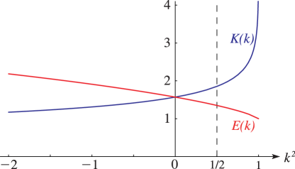
… ►See Figures 19.3.1–19.3.6 for complete and incomplete Legendre’s elliptic integrals. ►

See accompanying text — Figure 19.3.1: $K\left(k\right)$ and $E\left(k\right)$ as functions of $k^{2}$ for $-2\leq k^{2}\leq 1$ . Graphs of ${K^{\prime}}\left(k\right)$ and ${E^{\prime}}\left(k\right)$ are the mirror images in the vertical line $k^{2}=\frac{1}{2}$ . Magnify

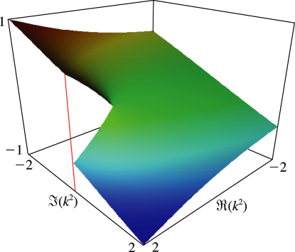
… ►In Figures 19.3.7 and 19.3.8 for complete Legendre’s elliptic integrals with complex arguments, height corresponds to the absolute value of the function and color to the phase. … ►

39: 29.8 Integral Equations

… ►Let

w(z)

be any solution of (29.2.1) of period

4K

w_{2}(z)

be a linearly independent solution, and

\mathscr{W}\left\{w,w_{2}\right\}

denote their Wronskian. … ►

29.8.1

x=k^{2}\operatorname{sn}\left(z,k\right)\operatorname{sn}\left(z_{1},k\right)% \operatorname{sn}\left(z_{2},k\right)\operatorname{sn}\left(z_{3},k\right)-% \frac{k^{2}}{{k^{\prime}}^{2}}\operatorname{cn}\left(z,k\right)\operatorname{% cn}\left(z_{1},k\right)\operatorname{cn}\left(z_{2},k\right)\operatorname{cn}% \left(z_{3},k\right)+\frac{1}{{k^{\prime}}^{2}}\operatorname{dn}\left(z,k% \right)\operatorname{dn}\left(z_{1},k\right)\operatorname{dn}\left(z_{2},k% \right)\operatorname{dn}\left(z_{3},k\right),

ⓘ

Symbols:: $\operatorname{cn}\left(\NVar{z},\NVar{k}\right)$ : Jacobian elliptic function, $\operatorname{dn}\left(\NVar{z},\NVar{k}\right)$ : Jacobian elliptic function, $\operatorname{sn}\left(\NVar{z},\NVar{k}\right)$ : Jacobian elliptic function, $x$ : real variable, $z$ : complex variable and $k$ : real parameter
Permalink:: http://dlmf.nist.gov/29.8.E1
Encodings:: pMML, png, TeX
See also:: Annotations for §29.8 and Ch.29

►where

z,z_{1},z_{2},z_{3}

are real, and

\operatorname{sn}

\operatorname{cn}

\operatorname{dn}

are the Jacobian elliptic functions (§22.2). … ►

w(z+2K)=\sigma w(z),

… ►

29.8.6

y=\frac{1}{k^{\prime}}\operatorname{dn}\left(z,k\right)\operatorname{dn}\left(% z_{1},k\right).

ⓘ

Symbols:: $\operatorname{dn}\left(\NVar{z},\NVar{k}\right)$ : Jacobian elliptic function, $y$ : real variable, $z$ : complex variable and $k$ : real parameter
Permalink:: http://dlmf.nist.gov/29.8.E6
Encodings:: pMML, png, TeX
See also:: Annotations for §29.8 and Ch.29

…

40: 36.1 Special Notation

… ►The main functions covered in this chapter are cuspoid catastrophes

\Phi_{K}\left(t;\mathbf{x}\right)

; umbilic catastrophes with codimension three

\Phi^{(\mathrm{E})}\left(s,t;\mathbf{x}\right)

\Phi^{(\mathrm{H})}\left(s,t;\mathbf{x}\right)

; canonical integrals

\Psi_{K}\left(\mathbf{x}\right)

\Psi^{(\mathrm{E})}\left(\mathbf{x}\right)

\Psi^{(\mathrm{H})}\left(\mathbf{x}\right)

; diffraction catastrophes

\Psi_{K}(\mathbf{x};k)

\Psi^{(\mathrm{E})}(\mathbf{x};k)

\Psi^{(\mathrm{H})}(\mathbf{x};k)

generated by the catastrophes. …