elliptical

SearchAdvancedHelp

(0.001 seconds)

21—30 of 169 matching pages

21: 19.13 Integrals of Elliptic Integrals

§19.13 Integrals of Elliptic Integrals

►

§19.13(i) Integration with Respect to the Modulus

… ►

§19.13(ii) Integration with Respect to the Amplitude

… ►

§19.13(iii) Laplace Transforms

►For direct and inverse Laplace transforms for the complete elliptic integrals $K\left(k\right)$, $E\left(k\right)$, and $D\left(k\right)$ see Prudnikov et al. (1992a, §3.31) and Prudnikov et al. (1992b, §§3.29 and 4.3.33), respectively.

22: 22.11 Fourier and Hyperbolic Series

§22.11 Fourier and Hyperbolic Series

… ►Similar expansions for ${\mathrm{cn}}^2(z,k)$ and ${\mathrm{dn}}^2(z,k)$ follow immediately from (22.6.1). … ►A related hyperbolic series is …Again, similar expansions for ${\mathrm{cn}}^2(z,k)$ and ${\mathrm{dn}}^2(z,k)$ may be derived via (22.6.1). …

23: 23.13 Zeros

§23.13 Zeros

…

24: 29.10 Lamé Functions with Imaginary Periods

… ►

29.10.2 $$z^{\prime }=\mathrm{i}(z-K-\mathrm{i}{K}^{\prime }),$$

ⓘ

Symbols:

$K^{\prime }\left(k\right)$: Legendre’s complementary complete elliptic integral of the first kind, $K\left(k\right)$: Legendre’s complete elliptic integral of the first kind, $\mathrm{i}$: imaginary unit, $z$: complex variable and $k$: real parameter

Permalink:

http://dlmf.nist.gov/29.10.E2

Encodings:

pMML, png, TeX

See also:

Annotations for §29.10 and Ch.29

… ►

${\mathrm{𝐸𝑐}}_{\nu }^{2m}(\mathrm{i}(z-K-\mathrm{i}{K}^{\prime }),k_{}^{\prime }{}_{}{}^2),$

►

${\mathrm{𝐸𝑐}}_{\nu }^{2m+1}(\mathrm{i}(z-K-\mathrm{i}{K}^{\prime }),k_{}^{\prime }{}_{}{}^2),$

►

${\mathrm{𝐸𝑠}}_{\nu }^{2m+1}(\mathrm{i}(z-K-\mathrm{i}{K}^{\prime }),k_{}^{\prime }{}_{}{}^2),$

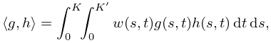
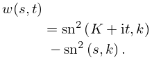
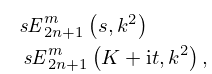
… ►The first and the fourth functions have period $2\mathrm{i}{K}^{\prime }$; the second and the third have period $4\mathrm{i}{K}^{\prime }$. …

25: 22.12 Expansions in Other Trigonometric Series and Doubly-Infinite Partial Fractions: Eisenstein Series

§22.12 Expansions in Other Trigonometric Series and Doubly-Infinite Partial Fractions: Eisenstein Series

… ►

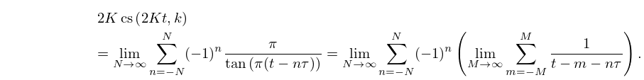
22.12.1 $$\tau =\mathrm{i}{K}^{\prime }\left(k\right)/K\left(k\right),$$

ⓘ

Symbols:

$K^{\prime }\left(k\right)$: Legendre’s complementary complete elliptic integral of the first kind, $K\left(k\right)$: Legendre’s complete elliptic integral of the first kind, $\mathrm{i}$: imaginary unit, $k$: modulus and $\tau$: ratio

Permalink:

http://dlmf.nist.gov/22.12.E1

Encodings:

pMML, png, TeX

See also:

Annotations for §22.12 and Ch.22

►

22.12.2 $$2Kk\mathrm{sn}(2Kt,k)=\sum _{n=-\mathrm{\infty }}^{\mathrm{\infty }}\frac{\pi }{\sin \left(\pi (t-(n+\frac{1}{2})\tau )\right)}=\sum _{n=-\mathrm{\infty }}^{\mathrm{\infty }}\left(\sum _{m=-\mathrm{\infty }}^{\mathrm{\infty }}\frac{{(-1)}^m}{t-m-(n+\frac{1}{2})\tau }\right),$$

ⓘ

Symbols:

$\mathrm{sn}(z,k)$: Jacobian elliptic function, $\pi$: the ratio of the circumference of a circle to its diameter, $K\left(k\right)$: Legendre’s complete elliptic integral of the first kind, $\sin z$: sine function, $k$: modulus and $\tau$: ratio

Referenced by:

§22.12, §22.12

Permalink:

http://dlmf.nist.gov/22.12.E2

Encodings:

pMML, png, TeX

See also:

Annotations for §22.12 and Ch.22

… ►

22.12.8 $$2K\mathrm{dc}(2Kt,k)=\sum _{n=-\mathrm{\infty }}^{\mathrm{\infty }}\frac{\pi }{\sin \left(\pi (t+\frac{1}{2}-n\tau )\right)}=\sum _{n=-\mathrm{\infty }}^{\mathrm{\infty }}\left(\sum _{m=-\mathrm{\infty }}^{\mathrm{\infty }}\frac{{(-1)}^m}{t+\frac{1}{2}-m-n\tau }\right),$$

ⓘ

Symbols:

$\mathrm{dc}(z,k)$: Jacobian elliptic function, $\pi$: the ratio of the circumference of a circle to its diameter, $K\left(k\right)$: Legendre’s complete elliptic integral of the first kind, $\sin z$: sine function, $k$: modulus and $\tau$: ratio

Permalink:

http://dlmf.nist.gov/22.12.E8

Encodings:

pMML, png, TeX

See also:

Annotations for §22.12 and Ch.22

… ►

22.12.13 $$2K\mathrm{cs}(2Kt,k)=\underset{N\to \mathrm{\infty }}{lim}\sum _{n=-N}^N{(-1)}^n\frac{\pi }{\tan \left(\pi (t-n\tau )\right)}=\underset{N\to \mathrm{\infty }}{lim}\sum _{n=-N}^N{(-1)}^n\left(\underset{M\to \mathrm{\infty }}{lim}\sum _{m=-M}^M\frac{1}{t-m-n\tau }\right).$$

ⓘ

Symbols:

$\mathrm{cs}(z,k)$: Jacobian elliptic function, $\pi$: the ratio of the circumference of a circle to its diameter, $K\left(k\right)$: Legendre’s complete elliptic integral of the first kind, $\tan z$: tangent function, $k$: modulus and $\tau$: ratio

Referenced by:

§22.12

Permalink:

http://dlmf.nist.gov/22.12.E13

Encodings:

pMML, png, TeX

See also:

Annotations for §22.12 and Ch.22

26: 19.4 Derivatives and Differential Equations

… ►

§19.4(i) Derivatives

… ►

${\displaystyle \frac{dE\left(k\right)}{dk}}={\displaystyle \frac{E\left(k\right)-K\left(k\right)}{k}},$

… ►

§19.4(ii) Differential Equations

… ►If $\varphi =\pi /2$, then these two equations become hypergeometric differential equations (15.10.1) for $K\left(k\right)$ and $E\left(k\right)$. An analogous differential equation of third order for $\mathrm{\Pi }(\varphi ,{\alpha }^2,k)$ is given in Byrd and Friedman (1971, 118.03).

27: 29.14 Orthogonality

… ►

29.14.2 $$⟨g,h⟩={\int }_0^K{\int }_0^{K^{\prime }}w(s,t)g(s,t)h(s,t)dtds,$$

ⓘ

Symbols:

$K^{\prime }\left(k\right)$: Legendre’s complementary complete elliptic integral of the first kind, $K\left(k\right)$: Legendre’s complete elliptic integral of the first kind, $dx$: differential of $x$ , $\int$: integral, $k$: real parameter and $w(s,t)$: function

Referenced by:

§29.14

Permalink:

http://dlmf.nist.gov/29.14.E2

Encodings:

pMML, png, TeX

See also:

Annotations for §29.14 and Ch.29

… ►

29.14.3 $$w(s,t)={\mathrm{sn}}^2(K+\mathrm{i}t,k)-{\mathrm{sn}}^2(s,k).$$

ⓘ

Symbols:

$\mathrm{sn}(z,k)$: Jacobian elliptic function, $K\left(k\right)$: Legendre’s complete elliptic integral of the first kind, $\mathrm{i}$: imaginary unit, $k$: real parameter and $w(s,t)$: function

Referenced by:

§29.14

Permalink:

http://dlmf.nist.gov/29.14.E3

Encodings:

pMML, png, TeX

See also:

Annotations for §29.14 and Ch.29

… ►

29.14.4 $${\mathrm{𝑠𝐸}}_{2n+1}^m(s,k^2){\mathrm{𝑠𝐸}}_{2n+1}^m(K+\mathrm{i}t,k^2),$$

ⓘ

Symbols:

${\mathrm{𝑠𝐸}}_{2n+1}^m(z,k^2)$: Lamé polynomial, $K\left(k\right)$: Legendre’s complete elliptic integral of the first kind, $\mathrm{i}$: imaginary unit, $m$: nonnegative integer, $n$: nonnegative integer and $k$: real parameter

Referenced by:

§29.14

Permalink:

http://dlmf.nist.gov/29.14.E4

Encodings:

pMML, png, TeX

See also:

Annotations for §29.14 and Ch.29

►

29.14.5 $${\mathrm{𝑐𝐸}}_{2n+1}^m(s,k^2){\mathrm{𝑐𝐸}}_{2n+1}^m(K+\mathrm{i}t,k^2),$$

ⓘ

Symbols:

${\mathrm{𝑐𝐸}}_{2n+1}^m(z,k^2)$: Lamé polynomial, $K\left(k\right)$: Legendre’s complete elliptic integral of the first kind, $\mathrm{i}$: imaginary unit, $m$: nonnegative integer, $n$: nonnegative integer and $k$: real parameter

Permalink:

http://dlmf.nist.gov/29.14.E5

Encodings:

pMML, png, TeX

See also:

Annotations for §29.14 and Ch.29

… ►

29.14.11 $$⟨g,h⟩={\int }_0^{4K}{\int }_0^{2K^{\prime }}w(s,t)g(s,t)h(s,t)dtds,$$

ⓘ

Symbols:

$K^{\prime }\left(k\right)$: Legendre’s complementary complete elliptic integral of the first kind, $K\left(k\right)$: Legendre’s complete elliptic integral of the first kind, $dx$: differential of $x$ , $\int$: integral, $k$: real parameter and $w(s,t)$: function

Permalink:

http://dlmf.nist.gov/29.14.E11

Encodings:

pMML, png, TeX

See also:

Annotations for §29.14 and Ch.29

…

28: 19.7 Connection Formulas

§19.7 Connection Formulas

… ►

Reciprocal-Modulus Transformation

… ►

Imaginary-Modulus Transformation

… ►

Imaginary-Argument Transformation

… ►

§19.7(iii) Change of Parameter of $\mathrm{\Pi }(\varphi ,{\alpha }^2,k)$

…

29: 19.6 Special Cases

§19.6 Special Cases

►

§19.6(i) Complete Elliptic Integrals

… ►Exact values of $K\left(k\right)$ and $E\left(k\right)$ for various special values of $k$ are given in Byrd and Friedman (1971, 111.10 and 111.11) and Cooper et al. (2006). ►

§19.6(ii) $F(\varphi ,k)$

… ►

§19.6(iii) $E(\varphi ,k)$

…

30: 29.13 Graphics

… ►

►►

Figure 29.13.5: ${\mathrm{𝑢𝐸}}_4^m(x,0.1)$ for $-2K\le x\le 2K$, $m=0,1,2$. $K=1.61244\mathrm{\dots }$. Magnify

►

►►

Figure 29.13.6: ${\mathrm{𝑢𝐸}}_4^m(x,0.9)$ for $-2K\le x\le 2K$, $m=0,1,2$. $K=2.57809\mathrm{\dots }$. Magnify

►

►►

Figure 29.13.7: ${\mathrm{𝑠𝐸}}_5^m(x,0.1)$ for $-2K\le x\le 2K$, $m=0,1,2$. $K=1.61244\mathrm{\dots }$. Magnify

►

►►

Figure 29.13.8: ${\mathrm{𝑠𝐸}}_5^m(x,0.9)$ for $-2K\le x\le 2K$, $m=0,1,2$. $K=2.57809\mathrm{\dots }$. Magnify

►

►►

Figure 29.13.9: ${\mathrm{𝑐𝐸}}_5^m(x,0.1)$ for $-2K\le x\le 2K$, $m=0,1,2$. $K=1.61244\mathrm{\dots }$. Magnify

…