elementary symmetric functions

(0.004 seconds)

1—10 of 24 matching pages

1: 19.36 Methods of Computation

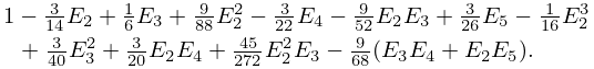
… ►When the differences are moderately small, the iteration is stopped, the elementary symmetric functions of certain differences are calculated, and a polynomial consisting of a fixed number of terms of the sum in (19.19.7) is evaluated. … ►

19.36.1

1-\tfrac{1}{10}E_{2}+\tfrac{1}{14}E_{3}+\tfrac{1}{24}E_{2}^{2}-\tfrac{3}{44}E_% {2}E_{3}-\tfrac{5}{208}E_{2}^{3}+\tfrac{3}{104}E_{3}^{2}+\tfrac{1}{16}E_{2}^{2% }E_{3},

ⓘ

Symbols:: $E_{s}(\mathbf{z})$ : symmetric function
Referenced by:: §19.19, §19.36(i), §19.36(i)
Permalink:: http://dlmf.nist.gov/19.36.E1
Encodings:: pMML, png, TeX
See also:: Annotations for §19.36(i), §19.36 and Ch.19

►where the elementary symmetric functions

E_{s}

are defined by (19.19.4). … ►

19.36.2

1-\tfrac{3}{14}E_{2}+\tfrac{1}{6}E_{3}+\tfrac{9}{88}E_{2}^{2}-\tfrac{3}{22}E_{% 4}-\tfrac{9}{52}E_{2}E_{3}+\tfrac{3}{26}E_{5}-\tfrac{1}{16}E_{2}^{3}+\tfrac{3}% {40}E_{3}^{2}+\tfrac{3}{20}E_{2}E_{4}+\tfrac{45}{272}E_{2}^{2}E_{3}-\tfrac{9}{% 68}(E_{3}E_{4}+E_{2}E_{5}).

ⓘ

Symbols:: $E_{s}(\mathbf{z})$ : symmetric function
Referenced by:: §19.19
Permalink:: http://dlmf.nist.gov/19.36.E2
Encodings:: pMML, png, TeX
See also:: Annotations for §19.36(i), §19.36 and Ch.19

… ►

19.36.4

\begin{aligned} z_{1}&=2.10985\;99098\;8,\\ z_{3}&=2.15673\;49098\;8,\\ Z_{1}&=0.00977\;77253\;5,\end{aligned}\quad\begin{aligned} z_{2}&=2.12548\;490% 98\;8,\\ A&=2.13069\;32432\;1,\\ Z_{2}&=0.00244\;44313\;4,\end{aligned}\\ {Z_{3}=-Z_{1}-Z_{2}=-0.01222\;21566\;9,}\\ {E_{2}=\Sci{-1.25480\;14}{-4},\quad E_{3}=\Sci{-2.9212}{-7}.}

ⓘ

Symbols:: $E_{s}(\mathbf{z})$ : symmetric function, $Z_{j}$ : components and $A$
Permalink:: http://dlmf.nist.gov/19.36.E4
Encodings:: pMML, png, TeX
See also:: Annotations for §19.36(i), §19.36(i), §19.36 and Ch.19

…

2: 19.19 Taylor and Related Series

… ►Define the elementary symmetric function

E_{s}(\mathbf{z})

by ►

19.19.4

\prod_{j=1}^{n}(1+tz_{j})=\sum_{s=0}^{n}t^{s}E_{s}(\mathbf{z}),

ⓘ

Defines:: $E_{s}(\mathbf{z})$ : symmetric function (locally)
Symbols:: $n$ : nonnegative integer
Referenced by:: §19.36(i)
Permalink:: http://dlmf.nist.gov/19.19.E4
Encodings:: pMML, png, TeX
See also:: Annotations for §19.19 and Ch.19

… ►

19.19.5

T_{N}(\mathbf{\tfrac{1}{2}},\mathbf{z})=\sum(-1)^{M+N}{\left(\tfrac{1}{2}% \right)_{M}}\frac{E_{1}^{m_{1}}(\mathbf{z})\cdots E_{n}^{m_{n}}(\mathbf{z})}{m% _{1}!\cdots m_{n}!},

ⓘ

Symbols:: ${\left(\NVar{a}\right)_{\NVar{n}}}$ : Pochhammer’s symbol (or shifted factorial), $!$ : factorial (as in $n!$ ), $m$ : nonnegative integer, $n$ : nonnegative integer, $N$ : nonnegative integer, $T_{N}(\mathbf{b},\mathbf{z})$ : polynomial, $E_{s}(\mathbf{z})$ : symmetric function and $M$ : sum
Referenced by:: §19.19, §19.36(i)
Permalink:: http://dlmf.nist.gov/19.19.E5
Encodings:: pMML, png, TeX
See also:: Annotations for §19.19 and Ch.19

… ►The number of terms in

T_{N}

can be greatly reduced by using variables

\mathbf{Z}=\boldsymbol{{1}}-(\mathbf{z}/A)

with

A

chosen to make

E_{1}(\mathbf{Z})=0

. … ►

E_{1}(\mathbf{Z})=0

|Z_{j}|<1

…

3: 19.15 Advantages of Symmetry

… ►Symmetry allows the expansion (19.19.7) in a series of elementary symmetric functions that gives high precision with relatively few terms and provides the most efficient method of computing the incomplete integral of the third kind (§19.36(i)). …

4: 1.11 Zeros of Polynomials

… ►The elementary symmetric functions of the zeros are (with

a_{n}\not=0

) …

5: 19.16 Definitions

… ►

§19.16(i) Symmetric Integrals

… ►Just as the elementary function

R_{C}\left(x,y\right)

(§19.2(iv)) is the degenerate case … ►

§19.16(ii) $R_{-a}\left(\mathbf{b};\mathbf{z}\right)$

… ► … ►

§19.16(iii) Various Cases of $R_{-a}\left(\mathbf{b};\mathbf{z}\right)$

…

6: Bibliography Z

… ►

R. Zanovello (1995) Numerical analysis of Struve functions with applications to other special functions. Ann. Numer. Math. 2 (1-4), pp. 199–208.

ⓘ

External Links:: ISSN 1021-2655, MathReview (F. W. J. Olver), ZentralBlatt
Referenced by:: §11.7(ii).
Encodings:: BibTeX

… ►

A. Zhedanov (1998) On some classes of polynomials orthogonal on arcs of the unit circle connected with symmetric orthogonal polynomials on an interval. J. Approx. Theory 94 (1), pp. 73–106.

ⓘ

External Links:: ISSN 0021-9045, Link, MathReview (T. S. Chihara), ZentralBlatt
Referenced by:: §18.33(iii).
Encodings:: BibTeX

… ►

D. G. Zill and B. C. Carlson (1970) Symmetric elliptic integrals of the third kind. Math. Comp. 24 (109), pp. 199–214.

ⓘ

External Links:: FullText, Document, MathReview (H. E. Fettis), ZentralBlatt
Referenced by:: §19.21(i), §19.21(iii), §19.22(iii), §19.25(i), §19.26(i).
Encodings:: BibTeX

►

A. Ziv (1991) Fast evaluation of elementary mathematical functions with correctly rounded last bit. ACM Trans. Math. Software 17 (3), pp. 410–423.

ⓘ

External Links:: ISSN 0098-3500, Document, ZentralBlatt
Referenced by:: §4.45(i).
Encodings:: BibTeX

►

I. J. Zucker (1979) The summation of series of hyperbolic functions. SIAM J. Math. Anal. 10 (1), pp. 192–206.

ⓘ

External Links:: ISSN 0036-1410, Document, MathReview (Y. L. Luke), ZentralBlatt
Referenced by:: §4.41.
Encodings:: BibTeX

…

7: 19.24 Inequalities

… ►

§19.24(i) Complete Integrals

►The condition

y\leq z

for (19.24.1) and (19.24.2) serves only to identify

y

as the smaller of the two nonzero variables of a symmetric function; it does not restrict validity. … ► ►

§19.24(ii) Incomplete Integrals

… ►The same reference also gives upper and lower bounds for symmetric integrals in terms of their elementary degenerate cases. …

8: 22.15 Inverse Functions

§22.15 Inverse Functions

… ►Each of these inverse functions is multivalued. … ►can be transformed into normal form by elementary change of variables. … ►For representations of the inverse functions as symmetric elliptic integrals see §19.25(v). …

9: 22.14 Integrals

… ►

§22.14(i) Indefinite Integrals of Jacobian Elliptic Functions

… ►For alternative, and symmetric, formulations of the results in this subsection see Carlson (2006a). … ►The indefinite integral of the 3rd power of a Jacobian function can be expressed as an elementary function of Jacobian functions and a product of Jacobian functions. … ►For indefinite integrals of squares and products of even powers of Jacobian functions in terms of symmetric elliptic integrals, see Carlson (2006b). … ► …

10: 19.17 Graphics

§19.17 Graphics

►See Figures 19.17.1–19.17.8 for symmetric elliptic integrals with real arguments. ►Because the

R

-function is homogeneous, there is no loss of generality in giving one variable the value

1

-1

(as in Figure 19.3.2). For

R_{F}

R_{G}

, and

R_{J}

, which are symmetric in

x, y, z

, we may further assume that

z

is the largest of

x, y, z

if the variables are real, then choose

z=1

, and consider only

0\leq x\leq 1

and

0\leq y\leq 1

. …The case

y=1

corresponds to elementary functions. …