eigenvalues of accessory parameter

SearchAdvancedHelp

(0.002 seconds)

21—30 of 415 matching pages

21: 29.15 Fourier Series and Chebyshev Series

… ►A convenient way of constructing the coefficients, together with the eigenvalues, is as follows. Equations (29.6.4), with $p=1,2,\mathrm{\dots },n$, (29.6.3), and $A_{2n+2}=0$ can be cast as an algebraic eigenvalue problem in the following way. …Let the eigenvalues of $𝐌$ be $H_p$ with … ►

29.15.7 $$a_{\nu }^{2m}\left(k^2\right)=\frac{1}{2}(H_m+\nu (\nu +1)k^2),$$

ⓘ

Symbols:

$a_{\nu }^n\left(k^2\right)$: eigenvalues of Lamé’s equation, $m$: nonnegative integer, $k$: real parameter, $\nu$: real parameter and $H_p$: eigenvalues

Permalink:

http://dlmf.nist.gov/29.15.E7

Encodings:

pMML, png, TeX

See also:

Annotations for §29.15(i), §29.15(i), §29.15 and Ch.29

… ►

29.15.22 $$a_{\nu }^{2m}\left(k^2\right)=\frac{1}{2}(H_m+\nu (\nu +1)k^2),$$

ⓘ

Symbols:

$a_{\nu }^n\left(k^2\right)$: eigenvalues of Lamé’s equation, $m$: nonnegative integer, $k$: real parameter, $\nu$: real parameter and $H_p$: eigenvalues

Permalink:

http://dlmf.nist.gov/29.15.E22

Encodings:

pMML, png, TeX

See also:

Annotations for §29.15(i), §29.15(i), §29.15 and Ch.29

…

22: 29.13 Graphics

… ►

§29.13(i) Eigenvalues for Lamé Polynomials

►

►►

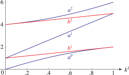
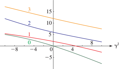
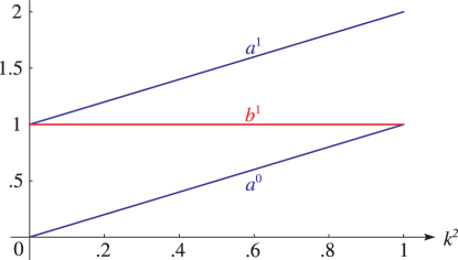
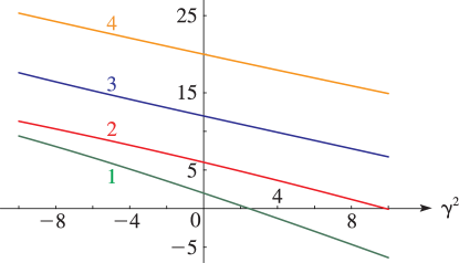
Figure 29.13.1: $a_2^m\left(k^2\right)$, $b_2^m\left(k^2\right)$ as functions of $k^2$ for $m=0,1,2$ ($a$’s), $m=1,2$ ($b$’s). Magnify

►

►►

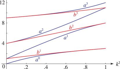
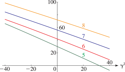
Figure 29.13.2: $a_1^m\left(k^2\right)$, $b_1^m\left(k^2\right)$ as functions of $k^2$ for $m=0,1$ ($a$’s), $m=1$ ($b$’s). Magnify

►

►►

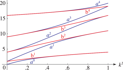
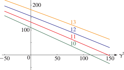
Figure 29.13.3: $a_3^m\left(k^2\right)$, $b_3^m\left(k^2\right)$ as functions of $k^2$ for $m=0,1,2,3$ ($a$’s), $m=1,2,3$ ($b$’s). Magnify

►

►►

Figure 29.13.4: $a_4^m\left(k^2\right)$, $b_4^m\left(k^2\right)$ as functions of $k^2$ for $m=0,1,2,3,4$ ($a$’s), $m=1,2,3,4$ ($b$’s). Magnify

…

23: 28.4 Fourier Series

… ►

$(a-4m^2)A_{2m}-q(A_{2m-2}+A_{2m+2})=0$ , $m=2,3,4,\mathrm{\dots }$, $a=a_{2n}\left(q\right)$, $A_{2m}=A_{2m}^{2n}(q)$.

… ►

28.4.24 $$\frac{A_{2m}^{2n}(q)}{A_0^{2n}(q)}=\frac{{(-1)}^m}{{(m!)}^2}{\left(\frac{q}{4}\right)}^m\frac{\pi \left(1+O\left(m^{-1}\right)\right)}{w_{\text{II}}(\frac{1}{2}\pi ;a_{2n}\left(q\right),q)},$$

ⓘ

Symbols:

$O\left(x\right)$: order not exceeding, $a_n\left(q\right)$: eigenvalues of Mathieu equation, $\pi$: the ratio of the circumference of a circle to its diameter, $!$: factorial (as in $n!$), $m$: integer, $q=h^2$: parameter, $n$: integer, $w_{\text{II}}(z;a,q)$: fundamental solution and $A_m(q)$: Fourier coefficient

Permalink:

http://dlmf.nist.gov/28.4.E24

Encodings:

pMML, png, TeX

See also:

Annotations for §28.4(vii), §28.4 and Ch.28

►

28.4.25 $$\frac{A_{2m+1}^{2n+1}(q)}{A_1^{2n+1}(q)}=\frac{{(-1)}^{m+1}}{{\left({\left(\frac{1}{2}\right)}_{m+1}\right)}^2}{\left(\frac{q}{4}\right)}^{m+1}\frac{2\left(1+O\left(m^{-1}\right)\right)}{w_{\text{II}}^{\prime }(\frac{1}{2}\pi ;a_{2n+1}\left(q\right),q)},$$

ⓘ

Symbols:

$O\left(x\right)$: order not exceeding, $a_n\left(q\right)$: eigenvalues of Mathieu equation, ${\left(a\right)}_n$: Pochhammer’s symbol (or shifted factorial), $\pi$: the ratio of the circumference of a circle to its diameter, $m$: integer, $q=h^2$: parameter, $n$: integer, $w(z)$: Mathieu’s equation solution and $A_m(q)$: Fourier coefficient

Permalink:

http://dlmf.nist.gov/28.4.E25

Encodings:

pMML, png, TeX

See also:

Annotations for §28.4(vii), §28.4 and Ch.28

►

28.4.26 $$\frac{B_{2m+1}^{2n+1}(q)}{B_1^{2n+1}(q)}=\frac{{(-1)}^m}{{\left({\left(\frac{1}{2}\right)}_{m+1}\right)}^2}{\left(\frac{q}{4}\right)}^{m+1}\frac{2\left(1+O\left(m^{-1}\right)\right)}{w_{\text{I}}(\frac{1}{2}\pi ;b_{2n+1}\left(q\right),q)},$$

ⓘ

Symbols:

$O\left(x\right)$: order not exceeding, $b_n\left(q\right)$: eigenvalues of Mathieu equation, ${\left(a\right)}_n$: Pochhammer’s symbol (or shifted factorial), $\pi$: the ratio of the circumference of a circle to its diameter, $m$: integer, $q=h^2$: parameter, $n$: integer, $w_{\text{I}}(z;a,q)$: fundamental solution and $B_m(q)$: Fourier coefficient

Permalink:

http://dlmf.nist.gov/28.4.E26

Encodings:

pMML, png, TeX

See also:

Annotations for §28.4(vii), §28.4 and Ch.28

►

28.4.27 $$\frac{B_{2m}^{2n+2}(q)}{B_2^{2n+2}(q)}=\frac{{(-1)}^m}{{(m!)}^2}{\left(\frac{q}{4}\right)}^m\frac{q\pi \left(1+O\left(m^{-1}\right)\right)}{w_{\text{I}}^{\prime }(\frac{1}{2}\pi ;b_{2n+2}\left(q\right),q)}.$$

ⓘ

Symbols:

$O\left(x\right)$: order not exceeding, $b_n\left(q\right)$: eigenvalues of Mathieu equation, $\pi$: the ratio of the circumference of a circle to its diameter, $!$: factorial (as in $n!$), $m$: integer, $q=h^2$: parameter, $n$: integer, $w(z)$: Mathieu’s equation solution and $B_m(q)$: Fourier coefficient

Permalink:

http://dlmf.nist.gov/28.4.E27

Encodings:

pMML, png, TeX

See also:

Annotations for §28.4(vii), §28.4 and Ch.28

…

24: 29.1 Special Notation

… ►All derivatives are denoted by differentials, not by primes. ►The main functions treated in this chapter are the eigenvalues $a_{\nu }^{2m}\left(k^2\right)$, $a_{\nu }^{2m+1}\left(k^2\right)$, $b_{\nu }^{2m+1}\left(k^2\right)$, $b_{\nu }^{2m+2}\left(k^2\right)$, the Lamé functions ${\mathrm{𝐸𝑐}}_{\nu }^{2m}(z,k^2)$, ${\mathrm{𝐸𝑐}}_{\nu }^{2m+1}(z,k^2)$, ${\mathrm{𝐸𝑠}}_{\nu }^{2m+1}(z,k^2)$, ${\mathrm{𝐸𝑠}}_{\nu }^{2m+2}(z,k^2)$, and the Lamé polynomials ${\mathrm{𝑢𝐸}}_{2n}^m(z,k^2)$, ${\mathrm{𝑠𝐸}}_{2n+1}^m(z,k^2)$, ${\mathrm{𝑐𝐸}}_{2n+1}^m(z,k^2)$, ${\mathrm{𝑑𝐸}}_{2n+1}^m(z,k^2)$, ${\mathrm{𝑠𝑐𝐸}}_{2n+2}^m(z,k^2)$, ${\mathrm{𝑠𝑑𝐸}}_{2n+2}^m(z,k^2)$, ${\mathrm{𝑐𝑑𝐸}}_{2n+2}^m(z,k^2)$, ${\mathrm{𝑠𝑐𝑑𝐸}}_{2n+3}^m(z,k^2)$. The notation for the eigenvalues and functions is due to Erdélyi et al. (1955, §15.5.1) and that for the polynomials is due to Arscott (1964b, §9.3.2). … ►Other notations that have been used are as follows: Ince (1940a) interchanges $a_{\nu }^{2m+1}\left(k^2\right)$ with $b_{\nu }^{2m+1}\left(k^2\right)$. … ►

$${(s_{\nu }^m(k^2))}^2=\frac{4}{\pi }{\int }_0^K{\left({\mathrm{𝐸𝑠}}_{\nu }^m(x,k^2)\right)}^{2}dx.$$

25: 30.9 Asymptotic Approximations and Expansions

§30.9 Asymptotic Approximations and Expansions

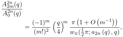
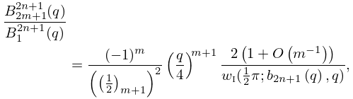
… ►For uniform asymptotic expansions in terms of Airy or Bessel functions for real values of the parameters, complex values of the variable, and with explicit error bounds see Dunster (1986). … ►The asymptotic behavior of ${\lambda }_n^m\left({\gamma }^2\right)$ and $a_{n,k}^m({\gamma }^2)$ as $n\to \mathrm{\infty }$ in descending powers of $2n+1$ is derived in Meixner (1944). …The behavior of ${\lambda }_n^m\left({\gamma }^2\right)$ for complex ${\gamma }^2$ and large $|{\lambda }_n^m\left({\gamma }^2\right)|$ is investigated in Hunter and Guerrieri (1982).

26: 29.20 Methods of Computation

… ►

§29.20(i) Lamé Functions

… ►Initial approximations to the eigenvalues can be found, for example, from the asymptotic expansions supplied in §29.7(i). … ►A third method is to approximate eigenvalues and Fourier coefficients of Lamé functions by eigenvalues and eigenvectors of finite matrices using the methods of §§3.2(vi) and 3.8(iv). … ►

§29.20(ii) Lamé Polynomials

►The eigenvalues corresponding to Lamé polynomials are computed from eigenvalues of the finite tridiagonal matrices $𝐌$ given in §29.15(i), using methods described in §3.2(vi) and Ritter (1998). …

27: 30.7 Graphics

… ►

§30.7(i) Eigenvalues

►

►►

Figure 30.7.1: Eigenvalues ${\lambda }_n^0\left({\gamma }^2\right)$, $n=0,1,2,3$, $-10\le {\gamma }^2\le 10$. Magnify

►

►►

Figure 30.7.2: Eigenvalues ${\lambda }_n^1\left({\gamma }^2\right)$ $n=1,2,3,4$, $-10\le {\gamma }^2\le 10$. Magnify

►

►►

Figure 30.7.3: Eigenvalues ${\lambda }_n^5\left({\gamma }^2\right)$, $n=5,6,7,8$, $-40\le {\gamma }^2\le 40$. Magnify

►

►►

Figure 30.7.4: Eigenvalues ${\lambda }_n^{10}\left({\gamma }^2\right)$, $n=10,11,12,13$, $-50\le {\gamma }^2\le 150$. Magnify

…

28: 28.29 Definitions and Basic Properties

… ►A generalization of Mathieu’s equation (28.2.1) is Hill’s equation … ►iff ${\mathrm{e}}^{\pi \mathrm{i}\nu }$ is an eigenvalue of the matrix … ►

§28.29(iii) Discriminant and Eigenvalues in the Real Case

… ►To every equation (28.29.1), there belong two increasing infinite sequences of real eigenvalues: … ►

28.29.17 $${\mu }_n,n=1,2,3,\mathrm{\dots },\text{ with }△({\mu }_n)=-2.$$

ⓘ

Defines:

${\mu }_n$: eigenvalues (locally)

Symbols:

$n$: integer

Referenced by:

§28.30(i)

Permalink:

http://dlmf.nist.gov/28.29.E17

Encodings:

pMML, png, TeX

See also:

Annotations for §28.29(iii), §28.29 and Ch.28

…

29: 29.9 Stability

… ►If $\nu$ is not an integer, then (29.2.1) is unstable iff $h\le a_{\nu }^0\left(k^2\right)$ or $h$ lies in one of the closed intervals with endpoints $a_{\nu }^m\left(k^2\right)$ and $b_{\nu }^m\left(k^2\right)$, $m=1,2,\mathrm{\dots }$. If $\nu$ is a nonnegative integer, then (29.2.1) is unstable iff $h\le a_{\nu }^0\left(k^2\right)$ or $h\in [b_{\nu }^m\left(k^2\right),a_{\nu }^m\left(k^2\right)]$ for some $m=1,2,\mathrm{\dots },\nu$.

30: 28.14 Fourier Series

… ►

28.14.1 $${\mathrm{me}}_{\nu }(z,q)=\sum _{m=-\mathrm{\infty }}^{\mathrm{\infty }}{c}_{2m}^{\nu }(q){\mathrm{e}}^{\mathrm{i}(\nu +2m)z},$$

ⓘ

Symbols:

${\mathrm{me}}_n(z,q)$: Mathieu function, $\mathrm{e}$: base of natural logarithm, $\mathrm{i}$: imaginary unit, $m$: integer, $q=h^2$: parameter, $z$: complex variable, $\nu$: complex parameter and $c_{2m}(q)$: coefficients

A&S Ref:

20.3.8 (in slightly different form)

Referenced by:

§28.22(ii)

Permalink:

http://dlmf.nist.gov/28.14.E1

Encodings:

pMML, png, TeX

See also:

Annotations for §28.14 and Ch.28

… ►

28.14.4 $$q{c}_{2m+2}-\left(a-{(\nu +2m)}^2\right)c_{2m}+q{c}_{2m-2}=0,$$ $a={\lambda }_{\nu }\left(q\right),c_{2m}=c_{2m}^{\nu }(q)$,

ⓘ

Symbols:

${\lambda }_{\nu +2n}\left(q\right)$: eigenvalues of Mathieu equation, $m$: integer, $q=h^2$: parameter, $\nu$: complex parameter, $a$: parameter and $c_{2m}(q)$: coefficients

Referenced by:

item (d), item (d)

Permalink:

http://dlmf.nist.gov/28.14.E4

Encodings:

pMML, png, TeX

See also:

Annotations for §28.14 and Ch.28

… ►

28.14.5 $$\sum _{m=-\mathrm{\infty }}^{\mathrm{\infty }}{\left(c_{2m}^{\nu }(q)\right)}^2=1;$$

ⓘ

Symbols:

$m$: integer, $q=h^2$: parameter, $\nu$: complex parameter and $c_{2m}(q)$: coefficients

Referenced by:

item (d)

Permalink:

http://dlmf.nist.gov/28.14.E5

Encodings:

pMML, png, TeX

See also:

Annotations for §28.14 and Ch.28

… ►

28.14.7 $$c_{-2m}^{-\nu }(q)=c_{2m}^{\nu }(q),$$

ⓘ

Symbols:

$m$: integer, $q=h^2$: parameter, $\nu$: complex parameter and $c_{2m}(q)$: coefficients

Permalink:

http://dlmf.nist.gov/28.14.E7

Encodings:

pMML, png, TeX

See also:

Annotations for §28.14 and Ch.28

►

28.14.8 $$c_{2m}^{\nu }(-q)={(-1)}^m{c}_{2m}^{\nu }(q).$$

ⓘ

Symbols:

$m$: integer, $q=h^2$: parameter, $\nu$: complex parameter and $c_{2m}(q)$: coefficients

Permalink:

http://dlmf.nist.gov/28.14.E8

Encodings:

pMML, png, TeX

See also:

Annotations for §28.14 and Ch.28

…