eigenvalues of accessory parameter

SearchAdvancedHelp

(0.002 seconds)

11—20 of 415 matching pages

11: 28.17 Stability as $x\to \pm \mathrm{\infty }$

§28.17 Stability as $x\to \pm \mathrm{\infty }$

►If all solutions of (28.2.1) are bounded when $x\to \pm \mathrm{\infty }$ along the real axis, then the corresponding pair of parameters $(a,q)$ is called stable. … ►The boundary of each region comprises the characteristic curves $a=a_n\left(q\right)$ and $a=b_n\left(q\right)$; compare Figure 28.2.1. ►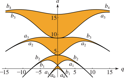

►►

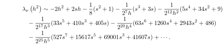
Figure 28.17.1: Stability chart for eigenvalues of Mathieu’s equation (28.2.1). Magnify

12: 28.16 Asymptotic Expansions for Large $q$

§28.16 Asymptotic Expansions for Large $q$

… ►

28.16.1 $${\lambda }_{\nu }\left(h^2\right)\sim -2h^2+2sh-\frac{1}{8}(s^2+1)-\frac{1}{2^{7}h}(s^3+3s)-\frac{1}{2^{12}{h}^2}(5s^4+34s^2+9)-\frac{1}{2^{17}{h}^3}(33s^5+410s^3+405s)-\frac{1}{2^{20}{h}^4}(63s^6+1260s^4+2943s^2+486)-\frac{1}{2^{25}{h}^5}(527s^7+15617s^5+69001s^3+41607s)+\mathrm{\cdots }.$$

ⓘ

Symbols:

${\lambda }_{\nu +2n}\left(q\right)$: eigenvalues of Mathieu equation, $\sim$: Poincaré asymptotic expansion, $h$: parameter and $\nu$: complex parameter

Permalink:

http://dlmf.nist.gov/28.16.E1

Encodings:

pMML, png, TeX

See also:

Annotations for §28.16 and Ch.28

…

13: 28.12 Definitions and Basic Properties

… ►

§28.12(i) Eigenvalues ${\lambda }_{\nu +2n}\left(q\right)$

… ►For given $\nu$ (or $\cos \left(\nu \pi \right)$) and $q$, equation (28.2.16) determines an infinite discrete set of values of $a$, denoted by ${\lambda }_{\nu +2n}\left(q\right)$, $n=0,\pm 1,\pm 2,\mathrm{\dots }$. …For other values of $q$, ${\lambda }_{\nu +2n}\left(q\right)$ is determined by analytic continuation. … … ►Two eigenfunctions correspond to each eigenvalue $a={\lambda }_{\nu }\left(q\right)$. …

14: 28.2 Definitions and Basic Properties

… ►

§28.2(v) Eigenvalues $a_n$, $b_n$

►For given $\nu$ and $q$, equation (28.2.16) determines an infinite discrete set of values of $a$, the eigenvalues or characteristic values, of Mathieu’s equation. … ►

Distribution

… ►

Change of Sign of $q$

… ►Table 28.2.2 gives the notation for the eigenfunctions corresponding to the eigenvalues in Table 28.2.1. …

15: 30.3 Eigenvalues

§30.3 Eigenvalues

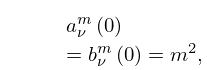
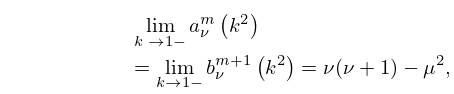
… ►These solutions exist only for eigenvalues ${\lambda }_n^m\left({\gamma }^2\right)$, $n=m,m+1,m+2,\mathrm{\dots }$, of the parameter $\lambda$. … ►

§30.3(iii) Transcendental Equation

… ►

§30.3(iv) Power-Series Expansion

… ►Further coefficients can be found with the Maple program SWF9; see §30.18(i).

16: 30.16 Methods of Computation

… ►

§30.16(i) Eigenvalues

… ►Approximations to eigenvalues can be improved by using the continued-fraction equations from §30.3(iii) and §30.8; see Bouwkamp (1947) and Meixner and Schäfke (1954, §3.93). … ►and real eigenvalues ${\alpha }_{1,d}$, ${\alpha }_{2,d}$, $\mathrm{\dots }$, ${\alpha }_{d,d}$, arranged in ascending order of magnitude. …The eigenvalues of $𝐀$ can be computed by methods indicated in §§3.2(vi), 3.2(vii). … ►which yields ${\lambda }_4^2\left(10\right)=\mathrm{13.97907\hspace{0.33em}345}$. …

17: 12.16 Mathematical Applications

… ►Sleeman (1968b) considers certain orthogonality properties of the PCFs and corresponding eigenvalues. In Brazel et al. (1992) exponential asymptotics are considered in connection with an eigenvalue problem involving PCFs. … ►PCFs are also used in integral transforms with respect to the parameter, and inversion formulas exist for kernels containing PCFs. …

18: 31.18 Methods of Computation

… ►The computation of the accessory parameter for the Heun functions is carried out via the continued-fraction equations (31.4.2) and (31.11.13) in the same way as for the Mathieu, Lamé, and spheroidal wave functions in Chapters 28–30.

19: 29.5 Special Cases and Limiting Forms

§29.5 Special Cases and Limiting Forms

►

29.5.1 $$a_{\nu }^m\left(0\right)=b_{\nu }^m\left(0\right)=m^2,$$

ⓘ

Symbols:

$a_{\nu }^n\left(k^2\right)$: eigenvalues of Lamé’s equation, $b_{\nu }^n\left(k^2\right)$: eigenvalues of Lamé’s equation, $m$: nonnegative integer and $\nu$: real parameter

Permalink:

http://dlmf.nist.gov/29.5.E1

Encodings:

pMML, png, TeX

See also:

Annotations for §29.5 and Ch.29

►

29.5.2 $${\mathrm{𝐸𝑐}}_{\nu }^0(z,0)=2^{-\frac{1}{2}},$$

ⓘ

Symbols:

${\mathrm{𝐸𝑐}}_{\nu }^m(z,k^2)$: Lamé function, $z$: complex variable and $\nu$: real parameter

Permalink:

http://dlmf.nist.gov/29.5.E2

Encodings:

pMML, png, TeX

See also:

Annotations for §29.5 and Ch.29

… ►Then ►

29.5.4 $$\underset{k\to 1-}{lim}{a}_{\nu }^m\left(k^2\right)=\underset{k\to 1-}{lim}{b}_{\nu }^{m+1}\left(k^2\right)=\nu (\nu +1)-{\mu }^2,$$

ⓘ

Symbols:

$a_{\nu }^n\left(k^2\right)$: eigenvalues of Lamé’s equation, $b_{\nu }^n\left(k^2\right)$: eigenvalues of Lamé’s equation, $m$: nonnegative integer, $k$: real parameter, $\nu$: real parameter and $\mu$: parameter

Permalink:

http://dlmf.nist.gov/29.5.E4

Encodings:

pMML, png, TeX

See also:

Annotations for §29.5 and Ch.29

…

20: 29.21 Tables

… ►

Ince (1940a) tabulates the eigenvalues $a_{\nu }^m\left(k^2\right)$, $b_{\nu }^{m+1}\left(k^2\right)$ (with $a_{\nu }^{2m+1}$ and $b_{\nu }^{2m+1}$ interchanged) for $k^2=0.1,0.5,0.9$, $\nu =-\frac{1}{2},0(1)25$, and $m=0,1,2,3$. Precision is 4D.

►

Arscott and Khabaza (1962) tabulates the coefficients of the polynomials $P$ in Table 29.12.1 (normalized so that the numerically largest coefficient is unity, i.e. monic polynomials), and the corresponding eigenvalues $h$ for $k^2=0.1(.1)0.9$, $n=1(1)30$. Equations from §29.6 can be used to transform to the normalization adopted in this chapter. Precision is 6S.