eigenvalues

SearchAdvancedHelp

(0.001 seconds)

21—30 of 87 matching pages

21: 28.35 Tables

§28.35 Tables

… ►

Blanch and Rhodes (1955) includes ${\mathrm{𝐵𝑒}}_n(t)$, ${\mathrm{𝐵𝑜}}_n(t)$, $t=\frac{1}{2}\sqrt{q}$, $n=0(1)15$; 8D. The range of $t$ is 0 to 0.1, with step sizes ranging from 0.002 down to 0.00025. Notation: ${\mathrm{𝐵𝑒}}_n(t)=a_n\left(q\right)+2q-(4n+2)\sqrt{q}$, ${\mathrm{𝐵𝑜}}_n(t)=b_n\left(q\right)+2q-(4n-2)\sqrt{q}$.

►

Ince (1932) includes eigenvalues $a_n$, $b_n$, and Fourier coefficients for $n=0$ or $1(1)6$, $q=0(1)10(2)20(4)40$; 7D. Also ${\mathrm{ce}}_n(x,q)$, ${\mathrm{se}}_n(x,q)$ for $q=0(1)10$, $x=1(1)90$, corresponding to the eigenvalues in the tables; 5D. Notation: $a_n={\mathrm{𝑏𝑒}}_n-2q$, $b_n={\mathrm{𝑏𝑜}}_n-2q$.

… ►

National Bureau of Standards (1967) includes the eigenvalues $a_n\left(q\right)$, $b_n\left(q\right)$ for $n=0(1)3$ with $q=0(.2)20(.5)37(1)100$, and $n=4(1)15$ with $q=0(2)100$; Fourier coefficients for ${\mathrm{ce}}_n(x,q)$ and ${\mathrm{se}}_n(x,q)$ for $n=0(1)15$, $n=1(1)15$, respectively, and various values of $q$ in the interval $[0,100]$; joining factors $g_{e,n}(\sqrt{q})$, $f_{e,n}(\sqrt{q})$ for $n=0(1)15$ with $q=0(.5\text{ to }10)100$ (but in a different notation). Also, eigenvalues for large values of $q$. Precision is generally 8D.

… ►

Blanch and Clemm (1969) includes eigenvalues $a_n\left(q\right)$, $b_n\left(q\right)$ for $q=\rho {\mathrm{e}}^{\mathrm{i}\varphi }$, $\rho =0(.5)25$, $\varphi =5^{\circ }(5^{\circ }){90}^{\circ }$, $n=0(1)15$; 4D. Also $a_n\left(q\right)$ and $b_n\left(q\right)$ for $q=\mathrm{i}\rho$, $\rho =0(.5)100$, $n=0(2)14$ and $n=2(2)16$, respectively; 8D. Double points for $n=0(1)15$; 8D. Graphs are included.

…

22: 30.16 Methods of Computation

… ►

§30.16(i) Eigenvalues

… ►Approximations to eigenvalues can be improved by using the continued-fraction equations from §30.3(iii) and §30.8; see Bouwkamp (1947) and Meixner and Schäfke (1954, §3.93). … ►and real eigenvalues ${\alpha }_{1,d}$, ${\alpha }_{2,d}$, $\mathrm{\dots }$, ${\alpha }_{d,d}$, arranged in ascending order of magnitude. …The eigenvalues of $𝐀$ can be computed by methods indicated in §§3.2(vi), 3.2(vii). … ►which yields ${\lambda }_4^2\left(10\right)=\mathrm{13.97907\hspace{0.33em}345}$. …

23: 12.16 Mathematical Applications

… ►Sleeman (1968b) considers certain orthogonality properties of the PCFs and corresponding eigenvalues. In Brazel et al. (1992) exponential asymptotics are considered in connection with an eigenvalue problem involving PCFs. …

24: 30.18 Software

… ►

SWF1: ${\lambda }_n^m\left({\gamma }^2\right)$.

… ►

§30.18(ii) Eigenvalues ${\lambda }_n^m\left({\gamma }^2\right)$

…

25: 30.17 Tables

§30.17 Tables

►

Stratton et al. (1956) tabulates quantities closely related to ${\lambda }_n^m\left({\gamma }^2\right)$ and $a_{n,k}^m({\gamma }^2)$ for $0\le m\le 8$, $m\le n\le 8$, $-64\le {\gamma }^2\le 64$. Precision is 7S.

►

Flammer (1957) includes 18 tables of eigenvalues, expansion coefficients, spheroidal wave functions, and other related quantities. Precision varies between 4S and 10S.

… ►

Van Buren et al. (1975) gives ${\lambda }_n^0\left({\gamma }^2\right)$, ${\mathrm{𝖯𝗌}}_n^0(x,{\gamma }^2)$ for $0\le n\le 49$, $-1600\le {\gamma }^2\le 1600$, $-1\le x\le 1$. Precision is 8S.

►

Zhang and Jin (1996) includes 24 tables of eigenvalues, spheroidal wave functions and their derivatives. Precision varies between 6S and 8S.

…

26: 3.2 Linear Algebra

… ►

§3.2(iv) Eigenvalues and Eigenvectors

… ► ►

§3.2(v) Condition of Eigenvalues

… ►has the same eigenvalues as $𝐀$. … ►

§3.2(vii) Computation of Eigenvalues

…

27: 29.5 Special Cases and Limiting Forms

§29.5 Special Cases and Limiting Forms

►

29.5.1 $$a_{\nu }^m\left(0\right)=b_{\nu }^m\left(0\right)=m^2,$$

ⓘ

Symbols:

$a_{\nu }^n\left(k^2\right)$: eigenvalues of Lamé’s equation, $b_{\nu }^n\left(k^2\right)$: eigenvalues of Lamé’s equation, $m$: nonnegative integer and $\nu$: real parameter

Permalink:

http://dlmf.nist.gov/29.5.E1

Encodings:

pMML, png, TeX

See also:

Annotations for §29.5 and Ch.29

… ►

29.5.4 $$\underset{k\to 1-}{lim}{a}_{\nu }^m\left(k^2\right)=\underset{k\to 1-}{lim}{b}_{\nu }^{m+1}\left(k^2\right)=\nu (\nu +1)-{\mu }^2,$$

ⓘ

Symbols:

$a_{\nu }^n\left(k^2\right)$: eigenvalues of Lamé’s equation, $b_{\nu }^n\left(k^2\right)$: eigenvalues of Lamé’s equation, $m$: nonnegative integer, $k$: real parameter, $\nu$: real parameter and $\mu$: parameter

Permalink:

http://dlmf.nist.gov/29.5.E4

Encodings:

pMML, png, TeX

See also:

Annotations for §29.5 and Ch.29

…

28: 28.36 Software

… ►

§28.36(ii) Characteristic Exponents and Eigenvalues

…

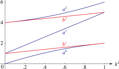
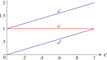
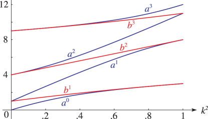
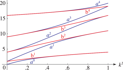
29: 29.13 Graphics

… ►

§29.13(i) Eigenvalues for Lamé Polynomials

►

►►

Figure 29.13.1: $a_2^m\left(k^2\right)$, $b_2^m\left(k^2\right)$ as functions of $k^2$ for $m=0,1,2$ ($a$’s), $m=1,2$ ($b$’s). Magnify

►

►►

Figure 29.13.2: $a_1^m\left(k^2\right)$, $b_1^m\left(k^2\right)$ as functions of $k^2$ for $m=0,1$ ($a$’s), $m=1$ ($b$’s). Magnify

►

►►

Figure 29.13.3: $a_3^m\left(k^2\right)$, $b_3^m\left(k^2\right)$ as functions of $k^2$ for $m=0,1,2,3$ ($a$’s), $m=1,2,3$ ($b$’s). Magnify

►

►►

Figure 29.13.4: $a_4^m\left(k^2\right)$, $b_4^m\left(k^2\right)$ as functions of $k^2$ for $m=0,1,2,3,4$ ($a$’s), $m=1,2,3,4$ ($b$’s). Magnify

…

30: 29.15 Fourier Series and Chebyshev Series

… ►A convenient way of constructing the coefficients, together with the eigenvalues, is as follows. Equations (29.6.4), with $p=1,2,\mathrm{\dots },n$, (29.6.3), and $A_{2n+2}=0$ can be cast as an algebraic eigenvalue problem in the following way. …Let the eigenvalues of $𝐌$ be $H_p$ with … ►

29.15.7 $$a_{\nu }^{2m}\left(k^2\right)=\frac{1}{2}(H_m+\nu (\nu +1)k^2),$$

ⓘ

Symbols:

$a_{\nu }^n\left(k^2\right)$: eigenvalues of Lamé’s equation, $m$: nonnegative integer, $k$: real parameter, $\nu$: real parameter and $H_p$: eigenvalues

Permalink:

http://dlmf.nist.gov/29.15.E7

Encodings:

pMML, png, TeX

See also:

Annotations for §29.15(i), §29.15(i), §29.15 and Ch.29

… ►

29.15.22 $$a_{\nu }^{2m}\left(k^2\right)=\frac{1}{2}(H_m+\nu (\nu +1)k^2),$$

ⓘ

Symbols:

$a_{\nu }^n\left(k^2\right)$: eigenvalues of Lamé’s equation, $m$: nonnegative integer, $k$: real parameter, $\nu$: real parameter and $H_p$: eigenvalues

Permalink:

http://dlmf.nist.gov/29.15.E22

Encodings:

pMML, png, TeX

See also:

Annotations for §29.15(i), §29.15(i), §29.15 and Ch.29

…