domperidone 10mg 365-RX.com/?id=1738

SearchAdvancedHelp

Did you mean dominione 10mg 365-becom/?id=1738 ?

(0.055 seconds)

1—10 of 193 matching pages

1: 10 Bessel Functions

Chapter 10 Bessel Functions

…

2: 14.33 Tables

… ►

Abramowitz and Stegun (1964, Chapter 8) tabulates ${𝖯}_n\left(x\right)$ for $n=0(1)3,9,10$, $x=0(.01)1$, 5–8D; ${𝖯}_n^{\prime }\left(x\right)$ for $n=1(1)4,9,10$, $x=0(.01)1$, 5–7D; ${𝖰}_n\left(x\right)$ and ${𝖰}_n^{\prime }\left(x\right)$ for $n=0(1)3,9,10$, $x=0(.01)1$, 6–8D; $P_n\left(x\right)$ and $P_n^{\prime }\left(x\right)$ for $n=0(1)5,9,10$, $x=1(.2)10$, 6S; $Q_n\left(x\right)$ and $Q_n^{\prime }\left(x\right)$ for $n=0(1)3,9,10$, $x=1(.2)10$, 6S. (Here primes denote derivatives with respect to $x$.)

►

Zhang and Jin (1996, Chapter 4) tabulates ${𝖯}_n\left(x\right)$ for $n=2(1)5,10$, $x=0(.1)1$, 7D; ${𝖯}_n\left(\cos \theta \right)$ for $n=1(1)4,10$, $\theta =0(5^{\circ }){90}^{\circ }$, 8D; ${𝖰}_n\left(x\right)$ for $n=0(1)2,10$, $x=0(.1)0.9$, 8S; ${𝖰}_n\left(\cos \theta \right)$ for $n=0(1)3,10$, $\theta =0(5^{\circ }){90}^{\circ }$, 8D; ${𝖯}_n^m\left(x\right)$ for $m=1(1)4$, $n-m=0(1)2$, $n=10$, $x=0,0.5$, 8S; ${𝖰}_n^m\left(x\right)$ for $m=1(1)4$, $n=0(1)2,10$, 8S; ${𝖯}_{\nu }^m\left(\cos \theta \right)$ for $m=0(1)3$, $\nu =0(.25)5$, $\theta =0({15}^{\circ }){90}^{\circ }$, 5D; $P_n\left(x\right)$ for $n=2(1)5,10$, $x=1(1)10$, 7S; $Q_n\left(x\right)$ for $n=0(1)2,10$, $x=2(1)10$, 8S. Corresponding values of the derivative of each function are also included, as are 6D values of the first 5 $\nu$-zeros of ${𝖯}_{\nu }^m\left(\cos \theta \right)$ and of its derivative for $m=0(1)4$, $\theta ={10}^{\circ },{30}^{\circ },{150}^{\circ }$.

… ►

Žurina and Karmazina (1964, 1965) tabulate the conical functions ${𝖯}_{-\frac{1}{2}+\mathrm{i}\tau }\left(x\right)$ for $\tau =0(.01)50$, $x=-0.9(.1)0.9$, 7S; $P_{-\frac{1}{2}+\mathrm{i}\tau }\left(x\right)$ for $\tau =0(.01)50$, $x=1.1(.1)2(.2)5(.5)10(10)60$, 7D. Auxiliary tables are included to facilitate computation for larger values of $\tau$ when .

►

Žurina and Karmazina (1963) tabulates the conical functions ${𝖯}_{-\frac{1}{2}+\mathrm{i}\tau }^1\left(x\right)$ for $\tau =0(.01)25$, $x=-0.9(.1)0.9$, 7S; $P_{-\frac{1}{2}+\mathrm{i}\tau }^1\left(x\right)$ for $\tau =0(.01)25$, $x=1.1(.1)2(.2)5(.5)10(10)60$, 7S. Auxiliary tables are included to assist computation for larger values of $\tau$ when .

…

3: 11 Struve and Related Functions

…

4: 19.38 Approximations

… ►Minimax polynomial approximations (§3.11(i)) for $K\left(k\right)$ and $E\left(k\right)$ in terms of $m=k^2$ with can be found in Abramowitz and Stegun (1964, §17.3) with maximum absolute errors ranging from 4×10⁻⁵ to 2×10⁻⁸. Approximations of the same type for $K\left(k\right)$ and $E\left(k\right)$ for are given in Cody (1965a) with maximum absolute errors ranging from 4×10⁻⁵ to 4×10⁻¹⁸. …

5: 8.26 Tables

… ►

Zhang and Jin (1996, Table 3.9) tabulates $I_x(a,b)$ for $x=0(.05)1$, $a=0.5,1,3,5,10$, $b=1,10$ to 8D.

… ►

Abramowitz and Stegun (1964, pp. 245–248) tabulates $E_n\left(x\right)$ for $n=2,3,4,10,20$, $x=0(.01)2$ to 7D; also $(x+n){\mathrm{e}}^x{E}_n\left(x\right)$ for $n=2,3,4,10,20$, $x^{-1}=0(.01)0.1(.05)0.5$ to 6S.

… ►

Pagurova (1961) tabulates $E_n\left(x\right)$ for $n=0(1)20$, $x=0(.01)2(.1)10$ to 4-9S; ${\mathrm{e}}^x{E}_n\left(x\right)$ for $n=2(1)10$, $x=10(.1)20$ to 7D; ${\mathrm{e}}^x{E}_p\left(x\right)$ for $p=0(.1)1$, $x=0.01(.01)7(.05)12(.1)20$ to 7S or 7D.

►

Stankiewicz (1968) tabulates $E_n\left(x\right)$ for $n=1(1)10$, $x=0.01(.01)5$ to 7D.

►

Zhang and Jin (1996, Table 19.1) tabulates $E_n\left(x\right)$ for $n=1,2,3,5,10,15,20$, $x=0(.1)1,1.5,2,3,5,10,20,30,50,100$ to 7D or 8S.

6: 12.19 Tables

… ►

Miller (1955) includes $W(a,x)$, $W(a,-x)$, and reduced derivatives for $a=-10(1)10$, $x=0(.1)10$, 8D or 8S. Modulus and phase functions, and also other auxiliary functions are tabulated.

►

Fox (1960) includes modulus and phase functions for $W(a,x)$ and $W(a,-x)$, and several auxiliary functions for $x^{-1}=0(.005)0.1$, $a=-10(1)10$, 8S.

►

Kireyeva and Karpov (1961) includes $D_p\left(x(1+\mathrm{i})\right)$ for $\pm x=0(.1)5$, $p=0(.1)2$, and $\pm x=5(.01)10$, $p=0(.5)2$, 7D.

►

Karpov and Čistova (1964) includes $D_p\left(x\right)$ for $p=-2(.1)0$, $\pm x=0(.01)5$; $p=-2(.05)0$, $\pm x=5(.01)10$, 6D.

… ►

Zhang and Jin (1996, pp. 455–473) includes $U(\pm n-\frac{1}{2},x)$, $V(\pm n-\frac{1}{2},x)$, $U(\pm \nu -\frac{1}{2},x)$, $V(\pm \nu -\frac{1}{2},x)$, and derivatives, $\nu =n+\frac{1}{2}$, $n=0(1)10(10)30$, $x=0.5,1,5,10,30,50$, 8S; $W(a,\pm x)$, $W(-a,\pm x)$, and derivatives, $a=h(1)5+h$, $x=0.5,1$ and $a=h(1)5+h$, $x=5$, $h=0,0.5$, 8S. Also, first zeros of $U(a,x)$, $V(a,x)$, and of derivatives, $a=-6(.5)-1$, 6D; first three zeros of $W(a,-x)$ and of derivative, $a=0(.5)4$, 6D; first three zeros of $W(-a,\pm x)$ and of derivative, $a=0.5(.5)5.5$, 6D; real and imaginary parts of $U(a,z)$, $a=-1.5(1)1.5$, $z=x+\mathrm{i}y$, $x=0.5,1,5,10$, $y=0(.5)10$, 8S.

…

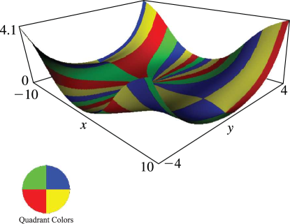
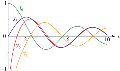
7: 10.3 Graphics

… ►

►►

Figure 10.3.1: $J_0\left(x\right)$, $Y_0\left(x\right)$, $J_1\left(x\right)$, $Y_1\left(x\right)$, $0\le x\le 10$. Magnify

… ►

►

►

Figure 10.3.9: $J_0\left(x+\mathrm{i}y\right)$, $-10\le x\le 10$, $-4\le y\le 4$. Magnify 3D Help

… ►

►

►

Figure 10.3.11: $J_1\left(x+\mathrm{i}y\right)$, $-10\le x\le 10$, $-4\le y\le 4$. Magnify 3D Help

… ►

►

►

Figure 10.3.13: $J_5\left(x+\mathrm{i}y\right)$, $-10\le x\le 10$, $-4\le y\le 4$. Magnify 3D Help

… ►

►

►

Figure 10.3.15: $J_{5.5}\left(x+\mathrm{i}y\right)$, $-10\le x\le 10$, $-4\le y\le 4$. … Magnify 3D Help

…

8: 29 Lamé Functions

…

9: 5.22 Tables

… ►Abramowitz and Stegun (1964, Chapter 6) tabulates $\mathrm{\Gamma }\left(x\right)$, $\ln \mathrm{\Gamma }\left(x\right)$, $\psi \left(x\right)$, and ${\psi }^{\prime }\left(x\right)$ for $x=1(.005)2$ to 10D; ${\psi }^{\prime \prime }\left(x\right)$ and ${\psi }^{(3)}\left(x\right)$ for $x=1(.01)2$ to 10D; $\mathrm{\Gamma }\left(n\right)$, $1/\mathrm{\Gamma }\left(n\right)$, $\mathrm{\Gamma }\left(n+\frac{1}{2}\right)$, $\psi \left(n\right)$, ${\log }_{10}\mathrm{\Gamma }\left(n\right)$, ${\log }_{10}\mathrm{\Gamma }\left(n+\frac{1}{3}\right)$, ${\log }_{10}\mathrm{\Gamma }\left(n+\frac{1}{2}\right)$, and ${\log }_{10}\mathrm{\Gamma }\left(n+\frac{2}{3}\right)$ for $n=1(1)101$ to 8–11S; $\mathrm{\Gamma }\left(n+1\right)$ for $n=100(100)1000$ to 20S. Zhang and Jin (1996, pp. 67–69 and 72) tabulates $\mathrm{\Gamma }\left(x\right)$, $1/\mathrm{\Gamma }\left(x\right)$, $\mathrm{\Gamma }\left(-x\right)$, $\ln \mathrm{\Gamma }\left(x\right)$, $\psi \left(x\right)$, $\psi \left(-x\right)$, ${\psi }^{\prime }\left(x\right)$, and ${\psi }^{\prime }\left(-x\right)$ for $x=0(.1)5$ to 8D or 8S; $\mathrm{\Gamma }\left(n+1\right)$ for $n=0(1)100(10)250(50)500(100)3000$ to 51S. … ►Abramowitz and Stegun (1964, Chapter 6) tabulates $\ln \mathrm{\Gamma }\left(x+\mathrm{i}y\right)$ for $x=1$ ($.1$) $2$, $y=0$ ($.1$) $10$ to 12D. …Zhang and Jin (1996, pp. 70, 71, and 73) tabulates the real and imaginary parts of $\mathrm{\Gamma }\left(x+\mathrm{i}y\right)$, $\ln \mathrm{\Gamma }\left(x+\mathrm{i}y\right)$, and $\psi \left(x+\mathrm{i}y\right)$ for $x=0.5,1,5,10$, $y=0(.5)10$ to 8S.

10: 18 Orthogonal Polynomials

…