completely multiplicative

SearchAdvancedHelp

(0.001 seconds)

1—10 of 16 matching pages

1: 27.3 Multiplicative Properties

… ►

27.3.8 $$\varphi \left(m\right)\varphi \left(n\right)=\varphi \left(mn\right)\varphi \left(\left(m,n\right)\right)/\left(m,n\right).$$

ⓘ

Symbols:

$\varphi \left(n\right)$: Euler’s totient, $\left(m,n\right)$: greatest common divisor (gcd), $m$: positive integer and $n$: positive integer

Permalink:

http://dlmf.nist.gov/27.3.E8

Encodings:

pMML, png, TeX

See also:

Annotations for §27.3 and Ch.27

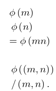
►A function $f$ is completely multiplicative if $f(1)=1$ and … ►If $f$ is completely multiplicative, then (27.3.2) becomes …

2: 27.20 Methods of Computation: Other Number-Theoretic Functions

… ►For a completely multiplicative function we use the values at the primes together with (27.3.10). …

3: 27.4 Euler Products and Dirichlet Series

… ►If $f(n)$ is completely multiplicative, then each factor in the product is a geometric series and the Euler product becomes … ►The completely multiplicative function $f(n)=n^{-s}$ gives the Euler product representation of the Riemann zeta function $\zeta \left(s\right)$ (§25.2(i)): …

4: 27.8 Dirichlet Characters

… ►If $k$ $(>1)$ is a given integer, then a function $\chi \left(n\right)$ is called a Dirichlet character (mod $k$) if it is completely multiplicative, periodic with period $k$, and vanishes when $\left(n,k\right)>1$. …

5: 22.8 Addition Theorems

… ►If sums/differences of the $z_j$’s are rational multiples of $K\left(k\right)$, then further relations follow. …

6: 22.5 Special Values

… ►Table 22.5.1 gives the value of each of the 12 Jacobian elliptic functions, together with its $z$-derivative (or at a pole, the residue), for values of $z$ that are integer multiples of $K$, $\mathrm{i}{K}^{\prime }$. …

7: 3.2 Linear Algebra

… ►To an eigenvalue of multiplicity $m$, there correspond $m$ linearly independent eigenvectors provided that $𝐀$ is nondefective, that is, $𝐀$ has a complete set of $n$ linearly independent eigenvectors. …

8: 1.18 Linear Second Order Differential Operators and Eigenfunction Expansions

… ►Such orthonormal sets are called complete. … ► … ►, of unit multiplicity, unless otherwise stated. …and completeness implies … ►and completeness relation …

9: 23.1 Special Notation

… ► ►►►►

$𝕃$	lattice in $ℂ$.
…
$K\left(k\right)$, $K^{\prime }\left(k\right)$	complete elliptic integrals (§19.2(i)).
…
$n\mathbb{Z}$	set of all integer multiples of $n$.
…

►The main functions treated in this chapter are the Weierstrass $\mathrm{\wp }$-function $\mathrm{\wp }\left(z\right)=\mathrm{\wp }\left(z|𝕃\right)=\mathrm{\wp }(z;g_2,g_3)$; the Weierstrass zeta function $\zeta \left(z\right)=\zeta \left(z|𝕃\right)=\zeta (z;g_2,g_3)$; the Weierstrass sigma function $\sigma \left(z\right)=\sigma \left(z|𝕃\right)=\sigma (z;g_2,g_3)$; the elliptic modular function $\lambda \left(\tau \right)$; Klein’s complete invariant $J\left(\tau \right)$; Dedekind’s eta function $\eta \left(\tau \right)$. …

10: Errata

… ►

17.6.1 $${}_2{}^{}\varphi _1^{}(\genfrac{}{}{0pt}{}{a,b}{c};q,c/(ab))=\frac{{(c/a,c/b;q)}_{\mathrm{\infty }}}{{(c,c/(ab);q)}_{\mathrm{\infty }}},$$

The constraint was added.

… ►

17.11.2 $${\mathrm{\Phi }}^{(2)}(a;b,b^{\prime };c,c^{\prime };q;x,y)=\frac{{(b,ax;q)}_{\mathrm{\infty }}}{{(c,x;q)}_{\mathrm{\infty }}}\sum _{n,r\geqq 0}\frac{{(a,b^{\prime };q)}_n{(c/b,x;q)}_r{b}^r{y}^n}{{(q,c^{\prime };q)}_n{(q;q)}_r{(ax;q)}_{n+r}}$$

The factor ${\left(q\right)}_r$ originally used in the denominator has been corrected to be ${(q;q)}_r$.

… ►

The multi-product notation ${(q,c;q)}_m{(q,c^{\prime };q)}_n$ in the denominator of the right-hand side was used.

… ►

17.2.22 $$\frac{{(q{a}^{\frac{1}{2}},-q{a}^{\frac{1}{2}};q)}_n}{{(a^{\frac{1}{2}},-a^{\frac{1}{2}};q)}_n}=\frac{{(a{q}^2;q^2)}_n}{{(a;q^2)}_n}=\frac{1-a{q}^{2n}}{1-a}$$

17.2.23 $$\frac{{(q{a}^{\frac{1}{k}},q{\omega }_k{a}^{\frac{1}{k}},\mathrm{\dots },q{\omega }_k^{k-1}{a}^{\frac{1}{k}};q)}_n}{{(a^{\frac{1}{k}},{\omega }_k{a}^{\frac{1}{k}},\mathrm{\dots },{\omega }_k^{k-1}{a}^{\frac{1}{k}};q)}_n}=\frac{{(a{q}^k;q^k)}_n}{{(a;q^k)}_n}=\frac{1-a{q}^{kn}}{1-a}$$

The numerators of the leftmost fractions were corrected to read ${(q{a}^{\frac{1}{2}},-q{a}^{\frac{1}{2}};q)}_n$ and ${(q{a}^{\frac{1}{k}},q{\omega }_k{a}^{\frac{1}{k}},\mathrm{\dots },q{\omega }_k^{k-1}{a}^{\frac{1}{k}};q)}_n$ instead of ${(q{a}^{\frac{1}{2}},-a{q}^{\frac{1}{2}};q)}_n$ and ${(a{q}^{\frac{1}{k}},q{\omega }_k{a}^{\frac{1}{k}},\mathrm{\dots },q{\omega }_k^{k-1}{a}^{\frac{1}{k}};q)}_n$, respectively.

Reported 2017-06-26 by Jason Zhao.

… ►

An addition was made to the Software Index to reflect a multiple precision (MP) package written in C++ which uses a variety of different MP interfaces. See Kormanyos (2011).

…