change of
(0.001 seconds)
31—40 of 120 matching pages
31: Errata
32: 12.11 Zeros
33: 4.16 Elementary Properties
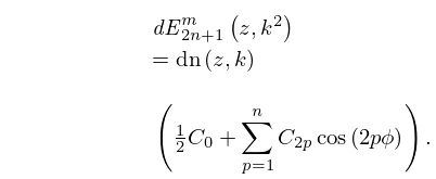
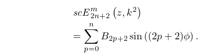
34: 29.15 Fourier Series and Chebyshev Series
35: 8.27 Approximations
…
►
•
…
DiDonato (1978) gives a simple approximation for the function (which is related to the incomplete gamma function by a change of variables) for real and large positive . This takes the form , approximately, where and is shown to produce an absolute error as .
36: Philip J. Davis
…
►The surface color map can be changed from height-based to phase-based for complex valued functions, and density plots can be generated through strategic scaling.
…
37: About the Project
…
►The former title of Associate Editor has been changed to Senior Associate Editor.
…
38: DLMF Project News
error generating summary39: 2.4 Contour Integrals
…
►The change of integration variable is given by
►
2.4.18
…
►
2.4.19
…
►By making a further change of variable
►
2.4.21
…
40: 2.3 Integrals of a Real Variable
…
►However, cancellation does not take place near the endpoints, owing to lack of symmetry, nor in the neighborhoods of zeros of because
changes relatively slowly at these stationary points.
…
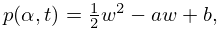
►A uniform approximation can be constructed by quadratic change of integration variable:
►
2.3.25
…
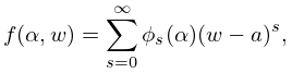
►
2.3.27
…
►
2.3.31
…
