bifurcation%20sets

SearchAdvancedHelp

(0.002 seconds)

11—20 of 606 matching pages

11: 10.75 Tables

… ►

The main tables in Abramowitz and Stegun (1964, Chapter 9) give $J_0\left(x\right)$ to 15D, $J_1\left(x\right)$, $J_2\left(x\right)$, $Y_0\left(x\right)$, $Y_1\left(x\right)$ to 10D, $Y_2\left(x\right)$ to 8D, $x=0(.1)17.5$; $Y_n\left(x\right)-(2/\pi )J_n\left(x\right)\ln x$, $n=0,1$, $x=0(.1)2$, 8D; $J_n\left(x\right)$, $Y_n\left(x\right)$, $n=3(1)9$, $x=0(.2)20$, 5D or 5S; $J_n\left(x\right)$, $Y_n\left(x\right)$, $n=0(1)20(10)50,100$, $x=1,2,5,10,50,100$, 10S; modulus and phase functions $\sqrt{x}{M}_n\left(x\right)$, ${\theta }_n\left(x\right)-x$, $n=0,1,2$, $1/x=0(.01)0.1$, 8D.

►

Achenbach (1986) tabulates $J_0\left(x\right)$, $J_1\left(x\right)$, $Y_0\left(x\right)$, $Y_1\left(x\right)$, $x=0(.1)8$, 20D or 18–20S.

… ►

Makinouchi (1966) tabulates all values of $j_{\nu ,m}$ and $y_{\nu ,m}$ in the interval $(0,100)$, with at least 29S. These are for $\nu =0(1)5$, 10, 20; $\nu =\frac{3}{2}$, $\frac{5}{2}$; $\nu =m/n$ with $m=1(1)n-1$ and $n=3(1)8$, except for $\nu =\frac{1}{2}$.

… ►

Bickley et al. (1952) tabulates $x^{-n}{I}_n\left(x\right)$ or ${\mathrm{e}}^{-x}{I}_n\left(x\right)$, $x^n{K}_n\left(x\right)$ or ${\mathrm{e}}^x{K}_n\left(x\right)$, $n=2(1)20$, $x=0$(.01 or .1) 10(.1) 20, 8S; $I_n\left(x\right)$, $K_n\left(x\right)$, $n=0(1)20$, $x=0$ or $0.1(.1)20$, 10S.

… ►

The main tables in Abramowitz and Stegun (1964, Chapter 9) give ${\mathrm{e}}^{-x}{I}_n\left(x\right)$, ${\mathrm{e}}^x{K}_n\left(x\right)$, $n=0,1,2$, $x=0(.1)10(.2)20$, 8D–10D or 10S; $\sqrt{x}{\mathrm{e}}^{-x}{I}_n\left(x\right)$, $(\sqrt{x}/\pi )$ ${\mathrm{e}}^x{K}_n\left(x\right)$, $n=0,1,2$, $1/x=0(.002)0.05$; $K_0\left(x\right)+I_0\left(x\right)\ln x$, $x(K_1\left(x\right)-I_1\left(x\right)\ln x)$, $x=0(.1)2$, 8D; ${\mathrm{e}}^{-x}{I}_n\left(x\right)$, ${\mathrm{e}}^x{K}_n\left(x\right)$, $n=3(1)9$, $x=0(.2)10(.5)20$, 5S; $I_n\left(x\right)$, $K_n\left(x\right)$, $n=0(1)20(10)50,100$, $x=1,2,5,10,50,100$, 9–10S.

…

12: 9.18 Tables

… ►

Miller (1946) tabulates $\mathrm{Ai}\left(x\right)$, ${\mathrm{Ai}}^{\prime }\left(x\right)$ for $x=-20(.01)2;$ ${\log }_{10}\mathrm{Ai}\left(x\right)$, ${\mathrm{Ai}}^{\prime }\left(x\right)/\mathrm{Ai}\left(x\right)$ for $x=0(.1)25(1)75$; $\mathrm{Bi}\left(x\right)$, ${\mathrm{Bi}}^{\prime }\left(x\right)$ for $x=-10(.1)2.5$; ${\log }_{10}\mathrm{Bi}\left(x\right)$, ${\mathrm{Bi}}^{\prime }\left(x\right)/\mathrm{Bi}\left(x\right)$ for $x=0(.1)10$; $M\left(x\right)$, $N\left(x\right)$, $\theta \left(x\right)$, $\varphi \left(x\right)$ (respectively $F(x)$, $G(x)$, $\chi (x)$, $\psi (x)$) for $x=-80(1)-30(.1)0$. Precision is generally 8D; slightly less for some of the auxiliary functions. Extracts from these tables are included in Abramowitz and Stegun (1964, Chapter 10), together with some auxiliary functions for large arguments.

►

Fox (1960, Table 3) tabulates $2{\pi }^{1/2}{x}^{1/4}\exp (\frac{2}{3}{x}^{3/2})\mathrm{Ai}\left(x\right)$, $2{\pi }^{1/2}{x}^{-1/4}\exp (\frac{2}{3}{x}^{3/2}){\mathrm{Ai}}^{\prime }\left(x\right)$, ${\pi }^{1/2}{x}^{1/4}\exp (-\frac{2}{3}{x}^{3/2})\mathrm{Bi}\left(x\right)$, and ${\pi }^{1/2}{x}^{-1/4}\exp (-\frac{2}{3}{x}^{3/2}){\mathrm{Bi}}^{\prime }\left(x\right)$ for $\frac{3}{2}{x}^{-3/2}=0(.001)0.05$, together with similar auxiliary functions for negative values of $x$. Precision is 10D.

►

Zhang and Jin (1996, p. 337) tabulates $\mathrm{Ai}\left(x\right)$, ${\mathrm{Ai}}^{\prime }\left(x\right)$, $\mathrm{Bi}\left(x\right)$, ${\mathrm{Bi}}^{\prime }\left(x\right)$ for $x=0(1)20$ to 8S and for $x=-20(1)0$ to 9D.

… ►

Miller (1946) tabulates $a_k$, ${\mathrm{Ai}}^{\prime }\left(a_k\right)$, $a_k^{\prime }$, $\mathrm{Ai}\left(a_k^{\prime }\right)$, $k=1(1)50$; $b_k$, ${\mathrm{Bi}}^{\prime }\left(b_k\right)$, $b_k^{\prime }$, $\mathrm{Bi}\left(b_k^{\prime }\right)$, $k=1(1)20$. Precision is 8D. Entries for $k=1(1)20$ are reproduced in Abramowitz and Stegun (1964, Chapter 10).

►

Sherry (1959) tabulates $a_k$, ${\mathrm{Ai}}^{\prime }\left(a_k\right)$, $a_k^{\prime }$, $\mathrm{Ai}\left(a_k^{\prime }\right)$, $k=1(1)50$; 20S.

…

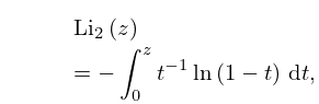
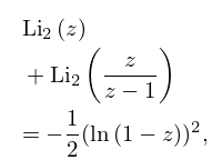
13: 25.12 Polylogarithms

… ►

25.12.2 $${\mathrm{Li}}_2\left(z\right)=-{\int }_0^z{t}^{-1}\ln \left(1-t\right)dt,$$ $z\in ℂ\setminus (1,\mathrm{\infty })$.

ⓘ

Symbols:

$ℂ$: complex plane, $dx$: differential of $x$ , ${\mathrm{Li}}_2\left(z\right)$: dilogarithm, $\in$: element of, $\int$: integral, $\ln z$: principal branch of logarithm function, $(a,b)$: open interval, $\setminus$: set subtraction, $x$: real variable and $z$: complex variable

Keywords:

definite integral, integral representation

Source:

Maximon (2003, (2.1), p. 2807)

A&S Ref:

27.7.1 (is a modified form with $z=1-x$)

Referenced by:

§25.12(i)

Permalink:

http://dlmf.nist.gov/25.12.E2

Encodings:

pMML, png, TeX

See also:

Annotations for §25.12(i), §25.12 and Ch.25

… ►

25.12.3 $${\mathrm{Li}}_2\left(z\right)+{\mathrm{Li}}_2\left(\frac{z}{z-1}\right)=-\frac{1}{2}{(\ln \left(1-z\right))}^2,$$ $z\in ℂ\setminus [1,\mathrm{\infty })$.

ⓘ

Symbols:

$[a,b)$: half-closed interval, $ℂ$: complex plane, ${\mathrm{Li}}_2\left(z\right)$: dilogarithm, $\in$: element of, $\ln z$: principal branch of logarithm function, $\setminus$: set subtraction, $x$: real variable and $z$: complex variable

Keywords:

connection formula

Source:

Maximon (2003, (3.4), p. 2808)

A&S Ref:

27.7.5 (is a modified form with $z=1-x$)

Permalink:

http://dlmf.nist.gov/25.12.E3

Encodings:

pMML, png, TeX

See also:

Annotations for §25.12(i), §25.12 and Ch.25

… ►

►►

Figure 25.12.1: Dilogarithm function ${\mathrm{Li}}_2\left(x\right)$, Magnify

►

►

►

Figure 25.12.2: Absolute value of the dilogarithm function $\left|{\mathrm{Li}}_2\left(x+\mathrm{i}y\right)\right|$, $-20\le x\le 20$, $-20\le y\le 20$. … Magnify 3D Help

… ►Sometimes the factor $1/\mathrm{\Gamma }\left(s+1\right)$ is omitted. …

14: 26.2 Basic Definitions

… ►A permutation is a one-to-one and onto function from a non-empty set to itself. If the set consists of the integers 1 through $n$, a permutation $\sigma$ can be thought of as a rearrangement of these integers where the integer in position $j$ is $\sigma (j)$. … ►Given a finite set $S$ with permutation $\sigma$, a cycle is an ordered equivalence class of elements of $S$ where $j$ is equivalent to $k$ if there exists an $\mathrm{\ell }=\mathrm{\ell }(j,k)$ such that $j={\sigma }^{\mathrm{\ell }}(k)$, where ${\sigma }^1=\sigma$ and ${\sigma }^{\mathrm{\ell }}$ is the composition of $\sigma$ with ${\sigma }^{\mathrm{\ell }-1}$. … ►

Partition

►A partition of a set $S$ is an unordered collection of pairwise disjoint nonempty sets whose union is $S$. …

15: 27.2 Functions

… ►Euclid’s Elements (Euclid (1908, Book IX, Proposition 20)) gives an elegant proof that there are infinitely many primes. … ►Gauss and Legendre conjectured that $\pi \left(x\right)$ is asymptotic to $x/\ln x$ as $x\to \mathrm{\infty }$: … ►Such a set is a reduced residue system modulo $n$. … ►

Table 27.2.2: Functions related to division.

► ►►►►

$n$	$\varphi \left(n\right)$	$d\left(n\right)$	$\sigma \left(n\right)$	$n$	$\varphi \left(n\right)$	$d\left(n\right)$	$\sigma \left(n\right)$	$n$	$\varphi \left(n\right)$	$d\left(n\right)$	$\sigma \left(n\right)$	$n$	$\varphi \left(n\right)$	$d\left(n\right)$	$\sigma \left(n\right)$
…
5	4	2	6	18	6	6	39	31	30	2	32	44	20	6	84
…
7	6	2	8	20	8	6	42	33	20	4	48	46	22	4	72
…

►

16: 25.20 Approximations

… ►

Cody et al. (1971) gives rational approximations for $\zeta \left(s\right)$ in the form of quotients of polynomials or quotients of Chebyshev series. The ranges covered are $0.5\le s\le 5$, $5\le s\le 11$, $11\le s\le 25$, $25\le s\le 55$. Precision is varied, with a maximum of 20S.

… ►

Antia (1993) gives minimax rational approximations for $\mathrm{\Gamma }\left(s+1\right)F_s(x)$, where $F_s(x)$ is the Fermi–Dirac integral (25.12.14), for the intervals and , with $s=-\frac{1}{2},\frac{1}{2},\frac{3}{2},\frac{5}{2}$. For each $s$ there are three sets of approximations, with relative maximum errors ${10}^{-4},{10}^{-8},{10}^{-12}$.

17: 26.4 Lattice Paths: Multinomial Coefficients and Set Partitions

§26.4 Lattice Paths: Multinomial Coefficients and Set Partitions

… ►(The empty set is considered to have one permutation consisting of no cycles.) $M_3$ is the number of set partitions of $\{1,2,\mathrm{\dots },n\}$ with $a_1$ subsets of size 1, $a_2$ subsets of size 2, $\mathrm{\dots }$, and $a_n$ subsets of size $n$: … ►

Table 26.4.1: Multinomials and partitions.

► ►►►

$n$	$m$	$\lambda$	$M_1$	$M_2$	$M_3$
…
$5$	$3$	$1^2,3^1$	$20$	$20$	$10$
…

►

…

18: 8 Incomplete Gamma and Related
Functions

…

19: 28 Mathieu Functions and Hill’s Equation

…

20: 26.13 Permutations: Cycle Notation

… ► ${𝔖}_n$ denotes the set of permutations of $\{1,2,\mathrm{\dots },n\}$. $\sigma \in {𝔖}_n$ is a one-to-one and onto mapping from $\{1,2,\mathrm{\dots },n\}$ to itself. … ►The number of elements of ${𝔖}_n$ with cycle type $\left(a_1,a_2,\mathrm{\dots },a_n\right)$ is given by (26.4.7). … ►The derangement number, $d(n)$, is the number of elements of ${𝔖}_n$ with no fixed points: … ►Given a permutation $\sigma \in {𝔖}_n$, the inversion number of $\sigma$, denoted $inv(\sigma )$, is the least number of adjacent transpositions required to represent $\sigma$. …