asymptotic formula

(0.003 seconds)

21—30 of 81 matching pages

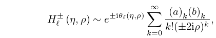
21: 33.11 Asymptotic Expansions for Large $\rho$

… ►

33.11.1

{H^{\pm}_{\ell}}\left(\eta,\rho\right)\sim e^{\pm\mathrm{i}{\theta_{\ell}}% \left(\eta,\rho\right)}\sum_{k=0}^{\infty}\frac{{\left(a\right)_{k}}{\left(b% \right)_{k}}}{k!(\pm 2\mathrm{i}\rho)^{k}},

ⓘ

Symbols:: ${\theta_{\NVar{\ell}}}\left(\NVar{\eta},\NVar{\rho}\right)$ : phase of Coulomb functions, ${\left(\NVar{a}\right)_{\NVar{n}}}$ : Pochhammer’s symbol (or shifted factorial), $\sim$ : Poincaré asymptotic expansion, $\mathrm{e}$ : base of natural logarithm, $!$ : factorial (as in $n!$ ), $\mathrm{i}$ : imaginary unit, ${H^{\NVar{\pm}}_{\NVar{\ell}}}\left(\NVar{\eta},\NVar{\rho}\right)$ : irregular Coulomb radial functions, $k$ : nonnegative integer, $\ell$ : nonnegative integer, $\rho$ : nonnegative real variable, $\eta$ : real parameter, $a$ : coefficient and $b$ : coefficient
A&S Ref:: 14.5.9
Referenced by:: Erratum (V1.0.19) for Equation (33.11.1), Erratum (V1.0.22) for Equation (33.11.1)
Permalink:: http://dlmf.nist.gov/33.11.E1
Encodings:: pMML, png, TeX
Errata (effective with 1.0.22):: Previously this formula was expressed as an equality. Since this formula expresses an asymptotic expansion, it has been corrected by using instead an $\sim$ relation.
Reported 2019-01-29 by Gergő Nemes
Errata (effective with 1.0.19):: Originally the factor in the denominator on the right-hand side was written incorrectly as $(\mp 2\mathrm{i}\rho)^{k}$ . This has been corrected to $(\pm 2\mathrm{i}\rho)^{k}$ .
Reported 2018-05-15 by Ian Thompson
See also:: Annotations for §33.11 and Ch.33

…

22: 2.2 Transcendental Equations

… ►where

F_{0}=f_{0}

and

sF_{s}

(

s\geq 1

) is the coefficient of

x^{-1}

in the asymptotic expansion of

(f(x))^{s}

(Lagrange’s formula for the reversion of series). …

23: 2.7 Differential Equations

… ►In combination with (2.7.14) these formulas yield asymptotic expansions for

w_{1}(z)

\frac{1}{2}\pi+\delta\leq\operatorname{ph}\left((\lambda_{2}-\lambda_{1})z% \right)\leq\frac{5}{2}\pi-\delta

, and

w_{2}(z)

-\frac{3}{2}\pi+\delta\leq\operatorname{ph}\left((\lambda_{2}-\lambda_{1})z% \right)\leq\frac{1}{2}\pi-\delta

. …

24: 29.20 Methods of Computation

… ►Initial approximations to the eigenvalues can be found, for example, from the asymptotic expansions supplied in §29.7(i). Subsequently, formulas typified by (29.6.4) can be applied to compute the coefficients of the Fourier expansions of the corresponding Lamé functions by backward recursion followed by application of formulas typified by (29.6.5) and (29.6.6) to achieve normalization; compare §3.6. … ►A fourth method is by asymptotic approximations by zeros of orthogonal polynomials of increasing degree. … ►§29.15(i) includes formulas for normalizing the eigenvectors. …

25: Errata

… ►

Expansion

§4.13 has been enlarged. The Lambert $W$ -function is multi-valued and we use the notation $W_{k}\left(x\right)$ , $k\in\mathbb{Z}$ , for the branches. The original two solutions are identified via $\operatorname{Wp}\left(x\right)=W_{0}\left(x\right)$ and $\operatorname{Wm}\left(x\right)=W_{\pm 1}\left(x\mp 0\mathrm{i}\right)$ .

Other changes are the introduction of the Wright $\omega$ -function and tree $T$ -function in (4.13.1_2) and (4.13.1_3), simplification formulas (4.13.3_1) and (4.13.3_2), explicit representation (4.13.4_1) for $\frac{{\mathrm{d}}^{n}W}{{\mathrm{d}z}^{n}}$ , additional Maclaurin series (4.13.5_1) and (4.13.5_2), an explicit expansion about the branch point at $z=-{\mathrm{e}}^{-1}$ in (4.13.9_1), extending the number of terms in asymptotic expansions (4.13.10) and (4.13.11), and including several integrals and integral representations for Lambert $W$ -functions in the end of the section.

… ►

Equation (33.11.1)

33.11.1

{H^{\pm}_{\ell}}\left(\eta,\rho\right)\sim{\mathrm{e}}^{\pm\mathrm{i}{\theta_{% \ell}}\left(\eta,\rho\right)}\sum_{k=0}^{\infty}\frac{{\left(a\right)_{k}}{% \left(b\right)_{k}}}{k!(\pm 2\mathrm{i}\rho)^{k}}

Previously this formula was expressed as an equality. Since this formula expresses an asymptotic expansion, it has been corrected by using instead an $\sim$ relation.

Reported by Gergő Nemes on 2019-01-29

… ►

Equation (5.11.8)

It was reported by Nico Temme on 2015-02-28 that the asymptotic formula for $\operatorname{Ln}\Gamma\left(z+h\right)$ is valid for $h$ $(\in\mathbb{C})$ ; originally it was unnecessarily restricted to $[0,1]$ .

…

26: 15.12 Asymptotic Approximations

… ►By combination of the foregoing results of this subsection with the linear transformations of §15.8(i) and the connection formulas of §15.10(ii), similar asymptotic approximations for

F\left(a+e_{1}\lambda,b+e_{2}\lambda;c+e_{3}\lambda;z\right)

can be obtained with

e_{j}=\pm 1

0

j=1,2,3

. …

27: 12.16 Mathematical Applications

… ►In Brazel et al. (1992) exponential asymptotics are considered in connection with an eigenvalue problem involving PCFs. ►PCFs are also used in integral transforms with respect to the parameter, and inversion formulas exist for kernels containing PCFs. …

28: 9.12 Scorer Functions

… ►For other phase ranges combine these results with the connection formulas (9.12.11)–(9.12.14) and the asymptotic expansions given in §9.7. …

29: 2.8 Differential Equations with a Parameter

… ►For results, including error bounds, see Olver (1977c). …

30: 10.74 Methods of Computation

… ►In the case of the spherical Bessel functions the explicit formulas given in §§10.49(i) and 10.49(ii) are terminating cases of the asymptotic expansions given in §§10.17(i) and 10.40(i) for the Bessel functions and modified Bessel functions. …