as z→0

SearchAdvancedHelp

(0.030 seconds)

11—20 of 616 matching pages

11: 22.5 Special Values

… ►For example, at $z=K+\mathrm{i}{K}^{\prime }$, $\mathrm{sn}(z,k)=1/k$, $d\mathrm{sn}(z,k)/dz=0$. … ►

Table 22.5.1: Jacobian elliptic function values, together with derivatives or residues, for special values of the variable.

► ►►►►►►

	$z$
…
$\mathrm{sn}z$	$0,1$	$1,0$	$1/k,0$	$\mathrm{\infty }$, $1/k$	$0,-1$	$0,-1$	$0,1$
…
$\mathrm{sd}z$	$0,1$	$k_{}^{\prime }{}_{}{}^{-1},0$	$\mathrm{\infty },-\mathrm{i}{(k{k}^{\prime })}^{-1}$	$\mathrm{i}{k}^{-1},0$	$0,-1$	$0,1$	$0,-1$
…
$\mathrm{dc}z$	$1,0$	$\mathrm{\infty },-1$	$0,k$	$k,0$	$-1,0$	$-1,0$	$1,0$
…
$\mathrm{sc}z$	$0,1$	$\mathrm{\infty },-k_{}^{\prime }{}_{}{}^{-1}$	$\mathrm{i}k_{}^{\prime }{}_{}{}^{-1},0$	$\mathrm{i},0$	$0,1$	$0,-1$	$0,-1$
…

►

…

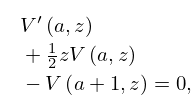
12: 16.8 Differential Equations

… ►is a value $z_0$ of $z$ at which all the coefficients $f_j(z)$, $j=0,1,\mathrm{\dots },n-1$, are analytic. If $z_0$ is not an ordinary point but ${(z-z_0)}^{n-j}{f}_j(z)$, $j=0,1,\mathrm{\dots },n-1$, are analytic at $z=z_0$, then $z_0$ is a regular singularity. … ►Equation (16.8.4) has a regular singularity at $z=0$, and an irregular singularity at $z=\mathrm{\infty }$, whereas (16.8.5) has regular singularities at $z=0$, $1$, and $\mathrm{\infty }$. … ►More generally if $z_0$ ($\in ℂ$) is an arbitrary constant, $|z-z_0|>\max (|z_0|,|z_0-1|)$, and , then …(Note that the generalized hypergeometric functions on the right-hand side are polynomials in $z_0$.) …

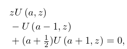
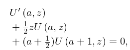
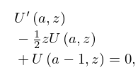
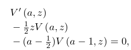
13: 12.8 Recurrence Relations and Derivatives

… ►

12.8.1 $$zU(a,z)-U(a-1,z)+(a+\frac{1}{2})U(a+1,z)=0,$$

ⓘ

Symbols:

$U(a,z)$: parabolic cylinder function, $z$: complex variable and $a$: real or complex parameter

A&S Ref:

19.6.4

Referenced by:

§12.8(i)

Permalink:

http://dlmf.nist.gov/12.8.E1

Encodings:

pMML, png, TeX

See also:

Annotations for §12.8(i), §12.8 and Ch.12

►

12.8.2 $$U^{\prime }(a,z)+\frac{1}{2}zU(a,z)+(a+\frac{1}{2})U(a+1,z)=0,$$

ⓘ

Symbols:

$U(a,z)$: parabolic cylinder function, $z$: complex variable and $a$: real or complex parameter

A&S Ref:

19.6.1

Permalink:

http://dlmf.nist.gov/12.8.E2

Encodings:

pMML, png, TeX

See also:

Annotations for §12.8(i), §12.8 and Ch.12

►

12.8.3 $$U^{\prime }(a,z)-\frac{1}{2}zU(a,z)+U(a-1,z)=0,$$

ⓘ

Symbols:

$U(a,z)$: parabolic cylinder function, $z$: complex variable and $a$: real or complex parameter

A&S Ref:

19.6.2

Permalink:

http://dlmf.nist.gov/12.8.E3

Encodings:

pMML, png, TeX

See also:

Annotations for §12.8(i), §12.8 and Ch.12

… ►

12.8.6 $$V^{\prime }(a,z)-\frac{1}{2}zV(a,z)-(a-\frac{1}{2})V(a-1,z)=0,$$

ⓘ

Symbols:

$V(a,z)$: parabolic cylinder function, $z$: complex variable and $a$: real or complex parameter

A&S Ref:

19.6.5

Permalink:

http://dlmf.nist.gov/12.8.E6

Encodings:

pMML, png, TeX

See also:

Annotations for §12.8(i), §12.8 and Ch.12

►

12.8.7 $$V^{\prime }(a,z)+\frac{1}{2}zV(a,z)-V(a+1,z)=0,$$

ⓘ

Symbols:

$V(a,z)$: parabolic cylinder function, $z$: complex variable and $a$: real or complex parameter

A&S Ref:

19.6.6

Permalink:

http://dlmf.nist.gov/12.8.E7

Encodings:

pMML, png, TeX

See also:

Annotations for §12.8(i), §12.8 and Ch.12

…

14: 36.5 Stokes Sets

… ►The Stokes set takes different forms for $z=0$, , and $z>0$. ►For $z=0$, the set consists of the two curves … ►For $z\ne 0$, the Stokes set is expressed in terms of scaled coordinates … ►For , there are two solutions $u$, provided that $|Y|>{(\frac{2}{5})}^{1/2}$. … ►For $z>0$ the Stokes set has two sheets. …

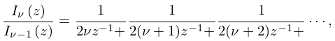
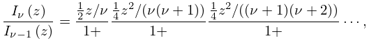
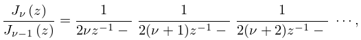
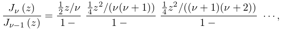
15: 10.33 Continued Fractions

… ►Assume $I_{\nu -1}\left(z\right)\ne 0$. … ►

10.33.1 $$\frac{I_{\nu }\left(z\right)}{I_{\nu -1}\left(z\right)}=\frac{1}{2\nu z^{-1}+}\frac{1}{2(\nu +1)z^{-1}+}\frac{1}{2(\nu +2)z^{-1}+}\mathrm{\cdots },$$ $z\ne 0$,

ⓘ

Symbols:

$I_{\nu }\left(z\right)$: modified Bessel function of the first kind, $z$: complex variable and $\nu$: complex parameter

Referenced by:

§10.74(v)

Permalink:

http://dlmf.nist.gov/10.33.E1

Encodings:

pMML, png, TeX

See also:

Annotations for §10.33 and Ch.10

►

10.33.2 $$\frac{I_{\nu }\left(z\right)}{I_{\nu -1}\left(z\right)}=\frac{\frac{1}{2}z/\nu }{1+}\frac{\frac{1}{4}{z}^2/(\nu (\nu +1))}{1+}\frac{\frac{1}{4}{z}^2/((\nu +1)(\nu +2))}{1+}\mathrm{\cdots },$$ $\nu \ne 0,-1,-2,\mathrm{\dots }$.

ⓘ

Symbols:

$I_{\nu }\left(z\right)$: modified Bessel function of the first kind, $z$: complex variable and $\nu$: complex parameter

Referenced by:

§10.74(v)

Permalink:

http://dlmf.nist.gov/10.33.E2

Encodings:

pMML, png, TeX

See also:

Annotations for §10.33 and Ch.10

…

16: 10.10 Continued Fractions

… ►Assume $J_{\nu -1}\left(z\right)\ne 0$. … ►

10.10.1 $$\frac{J_{\nu }\left(z\right)}{J_{\nu -1}\left(z\right)}=\frac{1}{2\nu z^{-1}-}\frac{1}{2(\nu +1)z^{-1}-}\frac{1}{2(\nu +2)z^{-1}-}\mathrm{\cdots },$$ $z\ne 0$,

ⓘ

Symbols:

$J_{\nu }\left(z\right)$: Bessel function of the first kind, $z$: complex variable and $\nu$: complex parameter

A&S Ref:

9.1.73

Referenced by:

§10.33, §10.74(v)

Permalink:

http://dlmf.nist.gov/10.10.E1

Encodings:

pMML, png, TeX

See also:

Annotations for §10.10 and Ch.10

►

10.10.2 $$\frac{J_{\nu }\left(z\right)}{J_{\nu -1}\left(z\right)}=\frac{\frac{1}{2}z/\nu }{1-}\frac{\frac{1}{4}{z}^2/(\nu (\nu +1))}{1-}\frac{\frac{1}{4}{z}^2/((\nu +1)(\nu +2))}{1-}\mathrm{\cdots },$$ $\nu \ne 0,-1,-2,\mathrm{\dots }$.

ⓘ

Symbols:

$J_{\nu }\left(z\right)$: Bessel function of the first kind, $z$: complex variable and $\nu$: complex parameter

A&S Ref:

9.1.73

Referenced by:

§10.33, §10.74(v)

Permalink:

http://dlmf.nist.gov/10.10.E2

Encodings:

pMML, png, TeX

See also:

Annotations for §10.10 and Ch.10

…

17: 3.7 Ordinary Differential Equations

… ►The path is partitioned at $P+1$ points labeled successively $z_0,z_1,\mathrm{\dots },z_P$, with $z_0=a$, $z_P=b$. … ►

$f_0(z)=1,$

►

$g_0(z)=0,$

►

$h_0(z)=0,$

… ►If the solution $w(z)$ that we are seeking grows in magnitude at least as fast as all other solutions of (3.7.1) as we pass along $𝒫$ from $a$ to $b$, then $w(z)$ and $w^{\prime }(z)$ may be computed in a stable manner for $z=z_0,z_1,\mathrm{\dots },z_P$ by successive application of (3.7.5) for $j=0,1,\mathrm{\dots },P-1$, beginning with initial values $w(a)$ and $w^{\prime }(a)$. …

18: 3.3 Interpolation

… ►The divided differences of $f$ relative to a sequence of distinct points $z_0,z_1,z_2,\mathrm{\dots }$ are defined by … ►Newton’s formula has the advantage of allowing easy updating: incorporation of a new point $z_{n+1}$ requires only addition of the term with $\left[z_0,z_1,\mathrm{\dots },z_{n+1}\right]f$ to (3.3.38), plus the computation of this divided difference. Another advantage is its robustness with respect to confluence of the set of points $z_0,z_1,\mathrm{\dots },z_n$. For example, for $k+1$ coincident points the limiting form is given by $\left[z_0,z_0,\mathrm{\dots },z_0\right]f=f^{(k)}(z_0)/k!$. … ►It can be used for solving a nonlinear scalar equation $f(z)=0$ approximately. …

19: 10.35 Generating Function and Associated Series

… ►For $z\in ℂ$ and $t\in ℂ\setminus \{0\}$, … ►

10.35.2 $${\mathrm{e}}^{z\cos \theta }=I_0\left(z\right)+2\sum _{k=1}^{\mathrm{\infty }}{I}_k\left(z\right)\cos \left(k\theta \right),$$

ⓘ

Symbols:

$\cos z$: cosine function, $\mathrm{e}$: base of natural logarithm, $I_{\nu }\left(z\right)$: modified Bessel function of the first kind, $k$: nonnegative integer and $z$: complex variable

A&S Ref:

9.6.34

Referenced by:

§10.35

Permalink:

http://dlmf.nist.gov/10.35.E2

Encodings:

pMML, png, TeX

See also:

Annotations for §10.35 and Ch.10

… ►

10.35.4 $$1=I_0\left(z\right)-2I_2\left(z\right)+2I_4\left(z\right)-2I_6\left(z\right)+\mathrm{\cdots },$$

ⓘ

Symbols:

$I_{\nu }\left(z\right)$: modified Bessel function of the first kind and $z$: complex variable

A&S Ref:

9.6.36

Permalink:

http://dlmf.nist.gov/10.35.E4

Encodings:

pMML, png, TeX

See also:

Annotations for §10.35 and Ch.10

►

10.35.5 $${\mathrm{e}}^{\pm z}=I_0\left(z\right)\pm 2I_1\left(z\right)+2I_2\left(z\right)\pm 2I_3\left(z\right)+\mathrm{\cdots },$$

ⓘ

Symbols:

$\mathrm{e}$: base of natural logarithm, $I_{\nu }\left(z\right)$: modified Bessel function of the first kind and $z$: complex variable

A&S Ref:

9.6.37,9.6.38

Permalink:

http://dlmf.nist.gov/10.35.E5

Encodings:

pMML, png, TeX

See also:

Annotations for §10.35 and Ch.10

►

$$\cosh z=I_0\left(z\right)+2I_2\left(z\right)+2I_4\left(z\right)+2I_6\left(z\right)+\mathrm{\dots },$$

…

20: 32.7 Bäcklund Transformations

… ►with $\zeta =-2^{1/3}z$ and $\epsilon =\pm 1$, where $W(\zeta ;\frac{1}{2}\epsilon )$ satisfies ${\text{P}}_{\text{II}}$ with $z=\zeta$, $\alpha =\frac{1}{2}\epsilon$, and $w(z;0)$ satisfies ${\text{P}}_{\text{II}}$ with $\alpha =0$. … ►Let $w_0=w(z;{\alpha }_0,{\beta }_0)$ and $w_j^{\pm }=w(z;{\alpha }_j^{\pm },{\beta }_j^{\pm })$, $j=1,2,3,4$, be solutions of ${\text{P}}_{\text{IV}}$ with … ►

$z_1=-z_0,$

►

$z_2=z_0,$

… ►Let $W_0=W(z;{\alpha }_0,{\beta }_0,{\gamma }_0,-\frac{1}{2})$ and $W_1=W(z;{\alpha }_1,{\beta }_1,{\gamma }_1,-\frac{1}{2})$ be solutions of ${\text{P}}_{\text{V}}$, where …