algebraic equations via Jacobian elliptic functions

SearchAdvancedHelp

(0.004 seconds)

11—20 of 980 matching pages

11: 19.16 Definitions

… ►

§19.16(i) Symmetric Integrals

… ►

§19.16(ii) $R_{-a}(𝐛;𝐳)$

►All elliptic integrals of the form (19.2.3) and many multiple integrals, including (19.23.6) and (19.23.6_5), are special cases of a multivariate hypergeometric function …The $R$-function is often used to make a unified statement of a property of several elliptic integrals. … ►

§19.16(iii) Various Cases of $R_{-a}(𝐛;𝐳)$

…

12: 5.2 Definitions

… ►

§5.2(i) Gamma and Psi Functions

►

Euler’s Integral

… ►It is a meromorphic function with no zeros, and with simple poles of residue ${(-1)}^n/n!$ at $z=-n$. … ►

5.2.6 $${\left(-a\right)}_n={(-1)}^n{\left(a-n+1\right)}_n,$$

ⓘ

Symbols:

${\left(a\right)}_n$: Pochhammer’s symbol (or shifted factorial), $n$: nonnegative integer and $a$: real or complex variable

Referenced by:

§5.2(iii), Erratum (V1.0.17) for Subsection 5.2(iii)

Permalink:

http://dlmf.nist.gov/5.2.E6

Encodings:

pMML, png, TeX

Addition (effective with 1.0.17):

This equation was added.

See also:

Annotations for §5.2(iii), §5.2 and Ch.5

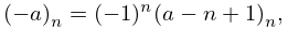
… ►Pochhammer symbols (rising factorials) ${\left(x\right)}_n=x(x+1)\mathrm{\cdots }(x+n-1)$ and falling factorials ${(-1)}^n{\left(-x\right)}_n=x(x-1)\mathrm{\cdots }(x-n+1)$ can be expressed in terms of each other via …

13: 31.1 Special Notation

… ►(For other notation see Notation for the Special Functions.) ► ►►

$x$, $y$	real variables.
…

►The main functions treated in this chapter are $H\mathrm{\ell }(a,q;\alpha ,\beta ,\gamma ,\delta ;z)$, $(s_1,s_2){\mathrm{𝐻𝑓}}_m(a,q_m;\alpha ,\beta ,\gamma ,\delta ;z)$, $(s_1,s_2){\mathrm{𝐻𝑓}}_m^{\nu }(a,q_m;\alpha ,\beta ,\gamma ,\delta ;z)$, and the polynomial ${\mathrm{𝐻𝑝}}_{n,m}(a,q_{n,m};-n,\beta ,\gamma ,\delta ;z)$. …Sometimes the parameters are suppressed.

14: 11.9 Lommel Functions

§11.9 Lommel Functions

… ►The inhomogeneous Bessel differential equation … ►For uniform asymptotic expansions, for large $\nu$ and fixed $\mu =-1,0,1,2,\mathrm{\dots }$, of solutions of the inhomogeneous modified Bessel differential equation that corresponds to (11.9.1) see Olver (1997b, pp. 388–390). … … ►

15: 15.2 Definitions and Analytical Properties

… ►

§15.2(i) Gauss Series

►The hypergeometric function $F(a,b;c;z)$ is defined by the Gauss series … … ►

§15.2(ii) Analytic Properties

… ►(Both interpretations give solutions of the hypergeometric differential equation (15.10.1), as does $𝐅(a,b;c;z)$, which is analytic at $c=0,-1,-2,\mathrm{\dots }$.) …

16: 9.12 Scorer Functions

§9.12 Scorer Functions

►

§9.12(i) Differential Equation

… ►Standard particular solutions are … ►

§9.12(iii) Initial Values

… ►

§9.12(iv) Numerically Satisfactory Solutions

…

17: 14.20 Conical (or Mehler) Functions

§14.20 Conical (or Mehler) Functions

►

§14.20(i) Definitions and Wronskians

… ► … ►

§14.20(ii) Graphics

… ►Approximations for ${𝖯}_{-\frac{1}{2}+\mathrm{i}\tau }^{\mu }\left(x\right)$ and ${\widehat{𝖰}}_{-\frac{1}{2}+\mathrm{i}\tau }^{-\mu }\left(x\right)$ can then be achieved via (14.9.7) and (14.20.3). …

18: 5.15 Polygamma Functions

§5.15 Polygamma Functions

►The functions ${\psi }^{(n)}\left(z\right)$, $n=1,2,\mathrm{\dots }$, are called the polygamma functions. In particular, ${\psi }^{\prime }\left(z\right)$ is the trigamma function; ${\psi }^{\prime \prime }$, ${\psi }^{(3)}$, ${\psi }^{(4)}$ are the tetra-, penta-, and hexagamma functions respectively. Most properties of these functions follow straightforwardly by differentiation of properties of the psi function. … ►For $B_{2k}$ see §24.2(i). …

19: 16.13 Appell Functions

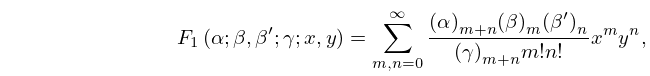
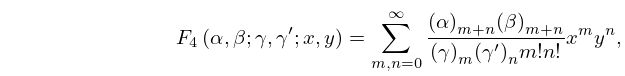
§16.13 Appell Functions

►The following four functions of two real or complex variables $x$ and $y$ cannot be expressed as a product of two ${}_2{}^{}F_1^{}$ functions, in general, but they satisfy partial differential equations that resemble the hypergeometric differential equation (15.10.1): ►

16.13.1 $$F_1(\alpha ;\beta ,{\beta }^{\prime };\gamma ;x,y)=\sum _{m,n=0}^{\mathrm{\infty }}\frac{{\left(\alpha \right)}_{m+n}{\left(\beta \right)}_m{\left({\beta }^{\prime }\right)}_n}{{\left(\gamma \right)}_{m+n}m!n!}{x}^m{y}^n,$$ ,

ⓘ

Defines:

$F_1(\alpha ;\beta ,{\beta }^{\prime };\gamma ;x,y)$: first Appell function

Symbols:

${\left(a\right)}_n$: Pochhammer’s symbol (or shifted factorial) and $!$: factorial (as in $n!$)

Permalink:

http://dlmf.nist.gov/16.13.E1

Encodings:

pMML, png, TeX

See also:

Annotations for §16.13 and Ch.16

… ►

16.13.4 $$F_4(\alpha ,\beta ;\gamma ,{\gamma }^{\prime };x,y)=\sum _{m,n=0}^{\mathrm{\infty }}\frac{{\left(\alpha \right)}_{m+n}{\left(\beta \right)}_{m+n}}{{\left(\gamma \right)}_m{\left({\gamma }^{\prime }\right)}_{n}m!n!}{x}^m{y}^n,$$ .

ⓘ

Defines:

$F_4(\alpha ,\beta ;\gamma ,{\gamma }^{\prime };x,y)$: fourth Appell function

Symbols:

${\left(a\right)}_n$: Pochhammer’s symbol (or shifted factorial) and $!$: factorial (as in $n!$)

Permalink:

http://dlmf.nist.gov/16.13.E4

Encodings:

pMML, png, TeX

See also:

Annotations for §16.13 and Ch.16

… ► …

20: 14.19 Toroidal (or Ring) Functions

§14.19 Toroidal (or Ring) Functions

►

§14.19(i) Introduction

… ►This form of the differential equation arises when Laplace’s equation is transformed into toroidal coordinates $(\eta ,\theta ,\varphi )$, which are related to Cartesian coordinates $(x,y,z)$ by … ►

§14.19(iv) Sums

… ►

§14.19(v) Whipple’s Formula for Toroidal Functions

…