Wilson polynomials

(0.003 seconds)

21—30 of 33 matching pages

21: 16.4 Argument Unity

… ►The characterizing properties (18.22.2), (18.22.10), (18.22.19), (18.22.20), and (18.26.14) of the Hahn and Wilson class polynomials are examples of the contiguous relations mentioned in the previous three paragraphs. …

22: Bibliography

… ►

R. Askey and J. Wilson (1985) Some basic hypergeometric orthogonal polynomials that generalize Jacobi polynomials. Mem. Amer. Math. Soc. 54 (319), pp. iv+55.

ⓘ

External Links:: ISSN 0065-9266, MathReview (Mourad E. H. Ismail), ZentralBlatt
Referenced by:: §18.21(ii), §18.22(ii), (18.28.24), §18.28(ii), Ch.18, Profile Richard A. Askey.
Encodings:: BibTeX

…

23: 18 Orthogonal Polynomials

Chapter 18 Orthogonal Polynomials

…

24: 18.27 $q$ -Hahn Class

… ►The $q$ -hypergeometric OP’s comprise the

q

-Hahn class (or

q

-linear lattice class) OP’s and the Askey–Wilson class (or

q

-quadratic lattice class) OP’s (§18.28). … ►

§18.27(ii) $q$ -Hahn Polynomials

… ►

§18.27(iii) Big $q$ -Jacobi Polynomials

… ►

§18.27(iv) Little $q$ -Jacobi Polynomials

… ►

Little $q$ -Laguerre polynomials

…

25: 18.22 Hahn Class: Recurrence Relations and Differences

… ►

§18.22(i) Recurrence Relations in $n$

… ►These polynomials satisfy (18.22.2) with

p_{n}(x)

A_{n}

, and

C_{n}

as in Table 18.22.1. ►

Table 18.22.1: Recurrence relations (18.22.2) for Krawtchouk, Meixner, and Charlier polynomials.

► ►►

$p_{n}(x)$	$A_{n}$	$C_{n}$
…

► … ►

§18.22(ii) Difference Equations in $x$

… ►

§18.22(iii) $x$ -Differences

…

26: 18.39 Applications in the Physical Sciences

… ►Derivations of (18.39.42) appear in Bethe and Salpeter (1957, pp. 12–20), and Pauling and Wilson (1985, Chapter V and Appendix VII), where the derivations are based on (18.39.36), and is also the notation of Piela (2014, §4.7), typifying the common use of the associated Coulomb–Laguerre polynomials in theoretical quantum chemistry. …

27: Bibliography P

… ►

A. M. Parkhurst and A. T. James (1974) Zonal Polynomials of Order

1

Through

12

. In Selected Tables in Mathematical Statistics, H. L. Harter and D. B. Owen (Eds.), Vol. 2, pp. 199–388.

ⓘ

External Links:: MathReview
Referenced by:: §35.11.
Encodings:: BibTeX

… ►

P. I. Pastro (1985) Orthogonal polynomials and some

q

-beta integrals of Ramanujan. J. Math. Anal. Appl. 112 (2), pp. 517–540.

ⓘ

External Links:: ISSN 0022-247X, Document, MathReview (Mourad E. H. Ismail), ZentralBlatt
Referenced by:: §18.33(iv), §18.33(v).
Encodings:: BibTeX

… ►

J. Patera and P. Winternitz (1973) A new basis for the representation of the rotation group. Lamé and Heun polynomials. J. Mathematical Phys. 14 (8), pp. 1130–1139.

ⓘ

External Links:: Document, ZentralBlatt
Referenced by:: §29.18(iv).
Encodings:: BibTeX

… ►

L. Pauling and E. B. Wilson (1985) Introduction to quantum mechanics. Dover Publications, Inc., New York.

ⓘ

Notes:: With applications to chemistry, Reprint of the 1935 original
External Links:: ISBN 0-486-64871-0, MathReview Entry
Referenced by:: §1.18(v), §18.39(i), §18.39(ii), §18.39(ii).
Encodings:: BibTeX

… ►

R. Piessens and M. Branders (1972) Chebyshev polynomial expansions of the Riemann zeta function. Math. Comp. 26 (120), pp. G1–G5.

ⓘ

External Links:: ISSN 0025-5718, FullText, MathReview
Referenced by:: 2nd item, 3rd item.
Encodings:: BibTeX

…

28: 18.19 Hahn Class: Definitions

§18.19 Hahn Class: Definitions

… ►

Wilson class (or quadratic lattice class). These are OP’s $p_{n}(x)=p_{n}(\lambda(y))$ ( $p_{n}(x)$ of degree $n$ in $x$ , $\lambda(y)$ quadratic in $y$ ) where the role of the differentiation operator is played by $\tfrac{\Delta_{y}}{\Delta_{y}(\lambda(y))}$ or $\tfrac{\nabla_{y}}{\nabla_{y}(\lambda(y))}$ or $\tfrac{\delta_{y}}{\delta_{y}(\lambda(y))}$ . The Wilson class consists of two discrete and two continuous families.

… ►

Hahn, Krawtchouk, Meixner, and Charlier

►Tables 18.19.1 and 18.19.2 provide definitions via orthogonality and standardization (§§18.2(i), 18.2(iii)) for the Hahn polynomials

Q_{n}\left(x;\alpha,\beta,N\right)

, Krawtchouk polynomials

K_{n}\left(x;p,N\right)

, Meixner polynomials

M_{n}\left(x;\beta,c\right)

, and Charlier polynomials

C_{n}\left(x;a\right)

. … ► …

29: Bibliography S

… ►

I. M. Sheffer (1939) Some properties of polynomial sets of type zero. Duke Math. J. 5, pp. 590–622.

ⓘ

External Links:: ISSN 0012-7094, Link, MathReview (A. Erdélyi), ZentralBlatt
Referenced by:: §18.2(xii).
Encodings:: BibTeX

… ►

A. Sri Ranga (2010) Szegő polynomials from hypergeometric functions. Proc. Amer. Math. Soc. 138 (12), pp. 4259–4270.

ⓘ

External Links:: ISSN 0002-9939, Link, MathReview (Andrei Martínez Finkelshtein), ZentralBlatt
Referenced by:: §18.33(iv).
Encodings:: BibTeX

… ►

W. F. Sun (1996) Uniform asymptotic expansions of Hermite polynomials. M. Phil. thesis, City University of Hong Kong.

ⓘ

External Links:: Abstract
Referenced by:: §18.16(v).
Encodings:: BibTeX

… ►

R. F. Swarttouw (1997) A computer implementation of the Askey-Wilson scheme. Technical Report 13 Vrije Universteit Amsterdam.

ⓘ

External Links:: FullText
Referenced by:: CAOP (website).
Encodings:: BibTeX

… ►

O. Szász (1950) On the relative extrema of ultraspherical polynomials. Boll. Un. Mat. Ital. (3) 5, pp. 125–127.

ⓘ

External Links:: MathReview (A. Erdélyi), ZentralBlatt
Referenced by:: §18.14(iii).
Encodings:: BibTeX

…

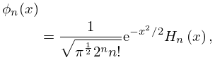
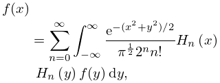
30: 1.18 Linear Second Order Differential Operators and Eigenfunction Expansions

… ►Writing Hermite’s differential equation (see Tables 18.3.1 and 18.8.1) in the form above, the eigenfunctions are

{\mathrm{e}}^{-x^{2}/2}H_{n}\left(x\right)

(

H_{n}

a Hermite polynomial,

n=0,1,2,\ldots

), with eigenvalues

\lambda_{n}=2n+1\in\boldsymbol{\sigma}_{p}

, for the differential operator … ►

1.18.42

\phi_{n}(x)=\frac{1}{\sqrt{{\pi}^{\frac{1}{2}}2^{n}n!}}{\mathrm{e}}^{-x^{2}/2}% H_{n}\left(x\right),

ⓘ

Symbols:: $H_{\NVar{n}}\left(\NVar{x}\right)$ : Hermite polynomial, $\pi$ : the ratio of the circumference of a circle to its diameter, $\mathrm{e}$ : base of natural logarithm, $!$ : factorial (as in $n!$ ) and $n$ : nonnegative integer
Permalink:: http://dlmf.nist.gov/1.18.E42
Encodings:: pMML, png, TeX
See also:: Annotations for §1.18(v), §1.18(v), §1.18 and Ch.1

… ►

1.18.43

f(x)=\sum_{n=0}^{\infty}\int_{-\infty}^{\infty}\frac{{\mathrm{e}}^{-(x^{2}+y^{% 2})/2}}{{\pi}^{\frac{1}{2}}2^{n}n!}H_{n}\left(x\right)H_{n}\left(y\right)f(y)% \,\mathrm{d}y,

ⓘ

Symbols:: $H_{\NVar{n}}\left(\NVar{x}\right)$ : Hermite polynomial, $\pi$ : the ratio of the circumference of a circle to its diameter, $\,\mathrm{d}\NVar{x}$ : differential of $x$ , $\mathrm{e}$ : base of natural logarithm, $!$ : factorial (as in $n!$ ), $\int$ : integral and $n$ : nonnegative integer
Permalink:: http://dlmf.nist.gov/1.18.E43
Encodings:: pMML, png, TeX
See also:: Annotations for §1.18(v), §1.18(v), §1.18 and Ch.1

… ►The implicit boundary conditions taken here are that the

\phi_{n}(x)

and

\phi_{n}^{\prime}(x)

vanish as

x\to\pm\infty

, which in this case is equivalent to requiring

\phi_{n}(x)\in L^{2}\left(X\right)

, see Pauling and Wilson (1985, pp. 67–82) for a discussion of this latter point. …