Whittaker functions

SearchAdvancedHelp

(0.006 seconds)

11—20 of 105 matching pages

11: 13.16 Integral Representations

… ►

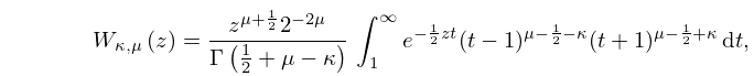
§13.16(i) Integrals Along the Real Line

… ►

13.16.5 $$W_{\kappa ,\mu }\left(z\right)=\frac{z^{\mu +\frac{1}{2}}{2}^{-2\mu }}{\mathrm{\Gamma }\left(\frac{1}{2}+\mu -\kappa \right)}{\int }_1^{\mathrm{\infty }}{\mathrm{e}}^{-\frac{1}{2}zt}{(t-1)}^{\mu -\frac{1}{2}-\kappa }{(t+1)}^{\mu -\frac{1}{2}+\kappa }dt,$$ $\mathrm{\Re }\mu +\frac{1}{2}>\mathrm{\Re }\kappa$, ,

ⓘ

Symbols:

$\mathrm{\Gamma }\left(z\right)$: gamma function, $W_{\kappa ,\mu }\left(z\right)$: Whittaker confluent hypergeometric function, $\pi$: the ratio of the circumference of a circle to its diameter, $dx$: differential of $x$ , $\mathrm{e}$: base of natural logarithm, $\int$: integral, $\mathrm{ph}$: phase, $\mathrm{\Re }$: real part and $z$: complex variable

Referenced by:

§13.29(iii)

Permalink:

http://dlmf.nist.gov/13.16.E5

Encodings:

pMML, png, TeX

See also:

Annotations for §13.16(i), §13.16 and Ch.13

… ► ►

§13.16(ii) Contour Integrals

… ►

§13.16(iii) Mellin–Barnes Integrals

…

12: 13.26 Addition and Multiplication Theorems

… ►

§13.26(i) Addition Theorems for $M_{\kappa ,\mu }\left(z\right)$

►The function $M_{\kappa ,\mu }\left(x+y\right)$ has the following expansions: … ►

§13.26(ii) Addition Theorems for $W_{\kappa ,\mu }\left(z\right)$

►The function $W_{\kappa ,\mu }\left(x+y\right)$ has the following expansions: … ►

§13.26(iii) Multiplication Theorems for $M_{\kappa ,\mu }\left(z\right)$ and $W_{\kappa ,\mu }\left(z\right)$

…

13: 33.14 Definitions and Basic Properties

… ►

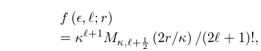
§33.14(ii) Regular Solution $f(ϵ,\mathrm{\ell };r)$

… ►

33.14.4 $$f(ϵ,\mathrm{\ell };r)={\kappa }^{\mathrm{\ell }+1}{M}_{\kappa ,\mathrm{\ell }+\frac{1}{2}}\left(2r/\kappa \right)/(2\mathrm{\ell }+1)!,$$

ⓘ

Defines:

$f(ϵ,\mathrm{\ell };r)$: regular Coulomb function

Symbols:

$M_{\kappa ,\mu }\left(z\right)$: Whittaker confluent hypergeometric function, $!$: factorial (as in $n!$), $\mathrm{\ell }$: nonnegative integer, $r$: real variable, $ϵ$: real parameter and $\kappa$: quantity

Referenced by:

§13.18(vi), (33.14.14)

Permalink:

http://dlmf.nist.gov/33.14.E4

Encodings:

pMML, png, TeX

See also:

Annotations for §33.14(ii), §33.14 and Ch.33

… ►

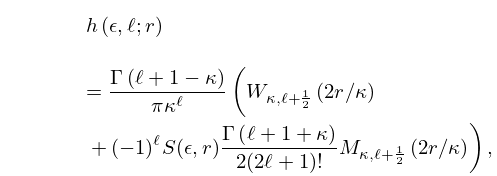
§33.14(iii) Irregular Solution $h(ϵ,\mathrm{\ell };r)$

… ►

33.14.7 $$h(ϵ,\mathrm{\ell };r)=\frac{\mathrm{\Gamma }\left(\mathrm{\ell }+1-\kappa \right)}{\pi {\kappa }^{\mathrm{\ell }}}\left(W_{\kappa ,\mathrm{\ell }+\frac{1}{2}}\left(2r/\kappa \right)+{(-1)}^{\mathrm{\ell }}S(ϵ,r)\frac{\mathrm{\Gamma }\left(\mathrm{\ell }+1+\kappa \right)}{2(2\mathrm{\ell }+1)!}{M}_{\kappa ,\mathrm{\ell }+\frac{1}{2}}\left(2r/\kappa \right)\right),$$

ⓘ

Defines:

$h(ϵ,\mathrm{\ell };r)$: irregular Coulomb function

Symbols:

$\mathrm{\Gamma }\left(z\right)$: gamma function, $M_{\kappa ,\mu }\left(z\right)$: Whittaker confluent hypergeometric function, $W_{\kappa ,\mu }\left(z\right)$: Whittaker confluent hypergeometric function, $\pi$: the ratio of the circumference of a circle to its diameter, $!$: factorial (as in $n!$), $\mathrm{\ell }$: nonnegative integer, $r$: real variable, $ϵ$: real parameter, $\kappa$: quantity and $S(ϵ,r)$: function

Referenced by:

§13.18(vi)

Permalink:

http://dlmf.nist.gov/33.14.E7

Encodings:

pMML, png, TeX

See also:

Annotations for §33.14(iii), §33.14 and Ch.33

… ►

33.14.14 $${\varphi }_{n,\mathrm{\ell }}(r)={(-1)}^{\mathrm{\ell }+1+n}{(2/n^3)}^{1/2}s(-1/n^2,\mathrm{\ell };r)=\frac{{(-1)}^{\mathrm{\ell }+1+n}}{n^{\mathrm{\ell }+2}}{\left(\frac{(n-\mathrm{\ell }-1)!}{(n+\mathrm{\ell })!}\right)}^{1/2}{(2r)}^{\mathrm{\ell }+1}{\mathrm{e}}^{-r/n}{L}_{n-\mathrm{\ell }-1}^{(2\mathrm{\ell }+1)}\left(2r/n\right)$$

ⓘ

Defines:

${\varphi }_{n,\mathrm{\ell }}(r)$: function (locally)

Symbols:

$s(ϵ,\mathrm{\ell };r)$: regular Coulomb function, $L_n^{(\alpha )}\left(x\right)$: Laguerre (or generalized Laguerre) polynomial, $\mathrm{e}$: base of natural logarithm, $!$: factorial (as in $n!$), $\mathrm{\ell }$: nonnegative integer and $r$: real variable

Referenced by:

(33.14.14), (33.14.15), §33.14(iv), §33.22(v), Erratum (V1.0.24) for Equation (33.14.15), Erratum (V1.0.24) for Subsection 33.14(iv)

Permalink:

http://dlmf.nist.gov/33.14.E14

Encodings:

pMML, png, TeX

Addition (effective with 1.0.24):

For the second equation in (33.14.14) first, via (33.14.9) and (33.14.4), express ${\varphi }_{n,\mathrm{\ell }}(r)$ in terms of Whittakerfunctions and then use (13.18.17).

See also:

Annotations for §33.14(iv), §33.14 and Ch.33

…

14: 33.2 Definitions and Basic Properties

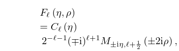
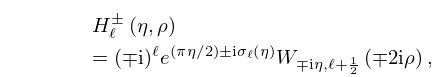
… ►The function $F_{\mathrm{\ell }}(\eta ,\rho )$ is recessive (§2.7(iii)) at $\rho =0$, and is defined by ►

33.2.3 $$F_{\mathrm{\ell }}(\eta ,\rho )=C_{\mathrm{\ell }}\left(\eta \right)2^{-\mathrm{\ell }-1}{(\mp \mathrm{i})}^{\mathrm{\ell }+1}{M}_{\pm \mathrm{i}\eta ,\mathrm{\ell }+\frac{1}{2}}\left(\pm 2\mathrm{i}\rho \right),$$

ⓘ

Defines:

$F_{\mathrm{\ell }}(\eta ,\rho )$: regular Coulomb radial function

Symbols:

$C_{\mathrm{\ell }}\left(\eta \right)$: normalizing constant for Coulomb radial functions, $M_{\kappa ,\mu }\left(z\right)$: Whittaker confluent hypergeometric function, $\mathrm{i}$: imaginary unit, $\mathrm{\ell }$: nonnegative integer, $\rho$: nonnegative real variable and $\eta$: real parameter

Referenced by:

§13.18(vi), §33.2(ii)

Permalink:

http://dlmf.nist.gov/33.2.E3

Encodings:

pMML, png, TeX

See also:

Annotations for §33.2(ii), §33.2 and Ch.33

… ►The functions $H_{\mathrm{\ell }}^{\pm }(\eta ,\rho )$ are defined by ►

33.2.7 $$H_{\mathrm{\ell }}^{\pm }(\eta ,\rho )={(\mp \mathrm{i})}^{\mathrm{\ell }}{\mathrm{e}}^{(\pi \eta /2)\pm \mathrm{i}{\sigma }_{\mathrm{\ell }}\left(\eta \right)}{W}_{\mp \mathrm{i}\eta ,\mathrm{\ell }+\frac{1}{2}}\left(\mp 2\mathrm{i}\rho \right),$$

ⓘ

Defines:

$H_{\mathrm{\ell }}^{\pm }(\eta ,\rho )$: irregular Coulomb radial functions

Symbols:

${\sigma }_{\mathrm{\ell }}\left(\eta \right)$: Coulomb phase shift, $W_{\kappa ,\mu }\left(z\right)$: Whittaker confluent hypergeometric function, $\pi$: the ratio of the circumference of a circle to its diameter, $\mathrm{e}$: base of natural logarithm, $\mathrm{i}$: imaginary unit, $\mathrm{\ell }$: nonnegative integer, $\rho$: nonnegative real variable and $\eta$: real parameter

Referenced by:

§13.18(vi), §33.23(vi)

Permalink:

http://dlmf.nist.gov/33.2.E7

Encodings:

pMML, png, TeX

See also:

Annotations for §33.2(iii), §33.2 and Ch.33

…

15: 12.1 Special Notation

… ►An older notation, due to Whittaker (1902), for $U(a,z)$ is $D_{\nu }\left(z\right)$. …

16: 33.16 Connection Formulas

… ►

§33.16(iii) $f$ and $h$ in Terms of $W_{\kappa ,\mu }\left(z\right)$ when

… ►

§33.16(v) $s$ and $c$ in Terms of $W_{\kappa ,\mu }\left(z\right)$ when

…

17: 8.5 Confluent Hypergeometric Representations

… ►For the confluent hypergeometric functions $M$, $𝐌$, $U$, and the Whittaker functions $M_{\kappa ,\mu }$ and $W_{\kappa ,\mu }$, see §§13.2(i) and 13.14(i). … ►

8.5.4 $$\gamma (a,z)=a^{-1}{z}^{\frac{1}{2}a-\frac{1}{2}}{\mathrm{e}}^{-\frac{1}{2}z}{M}_{\frac{1}{2}a-\frac{1}{2},\frac{1}{2}a}\left(z\right).$$

ⓘ

Symbols:

$M_{\kappa ,\mu }\left(z\right)$: Whittaker confluent hypergeometric function, $\mathrm{e}$: base of natural logarithm, $\gamma (a,z)$: incomplete gamma function, $z$: complex variable and $a$: parameter

Referenced by:

§8.5

Permalink:

http://dlmf.nist.gov/8.5.E4

Encodings:

pMML, png, TeX

See also:

Annotations for §8.5 and Ch.8

►

8.5.5 $$\mathrm{\Gamma }(a,z)={\mathrm{e}}^{-\frac{1}{2}z}{z}^{\frac{1}{2}a-\frac{1}{2}}{W}_{\frac{1}{2}a-\frac{1}{2},\frac{1}{2}a}\left(z\right).$$

ⓘ

Symbols:

$W_{\kappa ,\mu }\left(z\right)$: Whittaker confluent hypergeometric function, $\mathrm{e}$: base of natural logarithm, $\mathrm{\Gamma }(a,z)$: incomplete gamma function, $z$: complex variable and $a$: parameter

Permalink:

http://dlmf.nist.gov/8.5.E5

Encodings:

pMML, png, TeX

See also:

Annotations for §8.5 and Ch.8

18: 13.17 Continued Fractions

§13.17 Continued Fractions

… ►

13.17.1 $$\frac{\sqrt{z}{M}_{\kappa ,\mu }\left(z\right)}{M_{\kappa -\frac{1}{2},\mu +\frac{1}{2}}\left(z\right)}=1+\frac{u_{1}z}{1+}\frac{u_{2}z}{1+}\mathrm{\cdots },$$

ⓘ

Symbols:

$M_{\kappa ,\mu }\left(z\right)$: Whittaker confluent hypergeometric function, $z$: complex variable and $u_n$: continued fraction coefficients

Permalink:

http://dlmf.nist.gov/13.17.E1

Encodings:

pMML, png, TeX

See also:

Annotations for §13.17 and Ch.13

… ►

13.17.3 $$\frac{W_{\kappa ,\mu }\left(z\right)}{\sqrt{z}{W}_{\kappa -\frac{1}{2},\mu -\frac{1}{2}}\left(z\right)}=1+\frac{v_1/z}{1+}\frac{v_2/z}{1+}\mathrm{\cdots },$$

ⓘ

Symbols:

$W_{\kappa ,\mu }\left(z\right)$: Whittaker confluent hypergeometric function, $z$: complex variable and $v_n$: continued fraction coefficients

Permalink:

http://dlmf.nist.gov/13.17.E3

Encodings:

pMML, png, TeX

See also:

Annotations for §13.17 and Ch.13

…

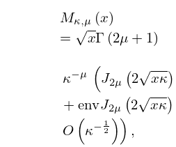
19: 13.21 Uniform Asymptotic Approximations for Large $\kappa$

§13.21 Uniform Asymptotic Approximations for Large $\kappa$

… ►

13.21.1 $$M_{\kappa ,\mu }\left(x\right)=\sqrt{x}\mathrm{\Gamma }\left(2\mu +1\right){\kappa }^{-\mu }\left(J_{2\mu }\left(2\sqrt{x\kappa }\right)+\mathrm{env}{J}_{2\mu }\left(2\sqrt{x\kappa }\right)O\left({\kappa }^{-\frac{1}{2}}\right)\right),$$

ⓘ

Symbols:

$J_{\nu }\left(z\right)$: Bessel function of the first kind, $O\left(x\right)$: order not exceeding, $\mathrm{\Gamma }\left(z\right)$: gamma function, $M_{\kappa ,\mu }\left(z\right)$: Whittaker confluent hypergeometric function, $\mathrm{env}{J}_{\nu }\left(x\right)$: envelope of Bessel function $J_{\nu }\left(x\right)$ and $x$: real variable

Permalink:

http://dlmf.nist.gov/13.21.E1

Encodings:

pMML, png, TeX

See also:

Annotations for §13.21(i), §13.21 and Ch.13

… ►

13.21.6 $$M_{-\kappa ,\mu }\left(4\kappa x\right)=\frac{2\mathrm{\Gamma }\left(2\mu +1\right)}{{\kappa }^{\mu -\frac{1}{2}}}{\left(\frac{x\zeta }{1+x}\right)}^{\frac{1}{4}}{I}_{2\mu }\left(4\kappa {\zeta }^{\frac{1}{2}}\right)\left(1+O\left({\kappa }^{-1}\right)\right),$$

ⓘ

Symbols:

$O\left(x\right)$: order not exceeding, $\mathrm{\Gamma }\left(z\right)$: gamma function, $M_{\kappa ,\mu }\left(z\right)$: Whittaker confluent hypergeometric function, $I_{\nu }\left(z\right)$: modified Bessel function of the first kind and $x$: real variable

Referenced by:

§13.21(i)

Permalink:

http://dlmf.nist.gov/13.21.E6

Encodings:

pMML, png, TeX

See also:

Annotations for §13.21(i), §13.21 and Ch.13

… ►For a uniform asymptotic expansion in terms of Airy functions for $W_{\kappa ,\mu }\left(4\kappa x\right)$ when $\kappa$ is large and positive, $\mu$ is real with $|\mu |$ bounded, and $x\in [\delta ,\mathrm{\infty })$ see Olver (1997b, Chapter 11, Ex. 7.3). … ►

20: 33.22 Particle Scattering and Atomic and Molecular Spectra

… ►For scattering problems, the interior solution is then matched to a linear combination of a pair of Coulomb functions, $F_{\mathrm{\ell }}(\eta ,\rho )$ and $G_{\mathrm{\ell }}(\eta ,\rho )$, or $f(ϵ,\mathrm{\ell };r)$ and $h(ϵ,\mathrm{\ell };r)$, to determine the scattering $S$-matrix and also the correct normalization of the interior wave solutions; see Bloch et al. (1951). ►For bound-state problems only the exponentially decaying solution is required, usually taken to be the Whittaker function $W_{-\eta ,\mathrm{\ell }+\frac{1}{2}}\left(2\rho \right)$. …