Weierstrass%E2%80%99s

SearchAdvancedHelp

(0.004 seconds)

11—20 of 622 matching pages

11: 23.1 Special Notation

… ► ►►►►►

$𝕃$	lattice in $ℂ$.
…
$={\mathrm{e}}^{\mathrm{i}\pi \tau }$	nome.
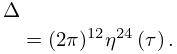
$\mathrm{\Delta }$	discriminant $g_2^3-27g_3^2$.
…
$S_1/S_2$	set of all elements of $S_1$, modulo elements of $S_2$. Thus two elements of $S_1/S_2$ are equivalent if they are both in $S_1$ and their difference is in $S_2$. (For an example see §20.12(ii).)
…

►The main functions treated in this chapter are the Weierstrass $\mathrm{\wp }$-function $\mathrm{\wp }\left(z\right)=\mathrm{\wp }\left(z|𝕃\right)=\mathrm{\wp }(z;g_2,g_3)$; the Weierstrass zeta function $\zeta \left(z\right)=\zeta \left(z|𝕃\right)=\zeta (z;g_2,g_3)$; the Weierstrass sigma function $\sigma \left(z\right)=\sigma \left(z|𝕃\right)=\sigma (z;g_2,g_3)$; the elliptic modular function $\lambda \left(\tau \right)$; Klein’s complete invariant $J\left(\tau \right)$; Dedekind’s eta function $\eta \left(\tau \right)$. …

12: 23.6 Relations to Other Functions

… ►

§23.6(i) Theta Functions

… ►

§23.6(ii) Jacobian Elliptic Functions

… ►

§23.6(iii) General Elliptic Functions

… ►

§23.6(iv) Elliptic Integrals

… ►

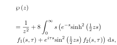
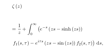
13: 23.11 Integral Representations

§23.11 Integral Representations

►Let $\tau ={\omega }_3/{\omega }_1$ and ►

$f_1(s,\tau )={\displaystyle \frac{{\cosh }^2\left(\frac{1}{2}\tau s\right)}{1-2{\mathrm{e}}^{-s}\cosh \left(\tau s\right)+{\mathrm{e}}^{-2s}}},$

… ►

23.11.2 $$\mathrm{\wp }\left(z\right)=\frac{1}{z^2}+8{\int }_0^{\mathrm{\infty }}s\left({\mathrm{e}}^{-s}{\sinh }^2\left(\frac{1}{2}zs\right)f_1(s,\tau )+{\mathrm{e}}^{\mathrm{i}\tau s}{\sin }^2\left(\frac{1}{2}zs\right)f_2(s,\tau )\right)ds,$$

ⓘ

Symbols:

$\mathrm{\wp }\left(z\right)$ (= $\mathrm{\wp }\left(z|𝕃\right)$ = $\mathrm{\wp }(z;g_2,g_3)$): Weierstrass $\mathrm{\wp }$-function, $dx$: differential of $x$ , $\mathrm{e}$: base of natural logarithm, $\sinh z$: hyperbolic sine function, $\mathrm{i}$: imaginary unit, $\int$: integral, $\sin z$: sine function, $𝕃$: lattice, $z$: complex, $\tau$: complex variable and $f_j(s,\tau )$: functions

Permalink:

http://dlmf.nist.gov/23.11.E2

Encodings:

pMML, png, TeX

See also:

Annotations for §23.11 and Ch.23

… ►

23.11.3 $$\zeta \left(z\right)=\frac{1}{z}+{\int }_0^{\mathrm{\infty }}\left({\mathrm{e}}^{-s}\left(zs-\sinh \left(zs\right)\right)f_1(s,\tau )-{\mathrm{e}}^{\mathrm{i}\tau s}\left(zs-\sin \left(zs\right)\right)f_2(s,\tau )\right)ds,$$

ⓘ

Symbols:

$\zeta \left(z\right)$ (= $\zeta \left(z|𝕃\right)$ = $\zeta (z;g_2,g_3)$): Weierstrass zeta function, $dx$: differential of $x$ , $\mathrm{e}$: base of natural logarithm, $\sinh z$: hyperbolic sine function, $\mathrm{i}$: imaginary unit, $\int$: integral, $\sin z$: sine function, $𝕃$: lattice, $z$: complex, $\tau$: complex variable and $f_j(s,\tau )$: functions

Permalink:

http://dlmf.nist.gov/23.11.E3

Encodings:

pMML, png, TeX

See also:

Annotations for §23.11 and Ch.23

…

14: 23.5 Special Lattices

… ►

§23.5(ii) Rectangular Lattice

… ►In this case the lattice roots $e_1$, $e_2$, and $e_3$ are real and distinct. … ►

§23.5(iii) Lemniscatic Lattice

… ►

§23.5(iv) Rhombic Lattice

… ►

§23.5(v) Equianharmonic Lattice

…

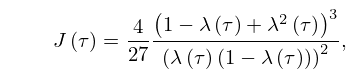
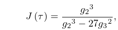
15: 23.19 Interrelations

… ►

23.19.1 $$\lambda \left(\tau \right)=16{\left(\frac{{\eta }^2\left(2\tau \right)\eta \left(\frac{1}{2}\tau \right)}{{\eta }^3\left(\tau \right)}\right)}^8,$$

ⓘ

Symbols:

$\eta \left(\tau \right)$: Dedekind’s eta function (or Dedekind modular function), $\lambda \left(\tau \right)$: elliptic modular function and $\tau$: complex variable

Permalink:

http://dlmf.nist.gov/23.19.E1

Encodings:

pMML, png, TeX

See also:

Annotations for §23.19 and Ch.23

►

23.19.2 $$J\left(\tau \right)=\frac{4}{27}\frac{{\left(1-\lambda \left(\tau \right)+{\lambda }^2\left(\tau \right)\right)}^3}{{\left(\lambda \left(\tau \right)\left(1-\lambda \left(\tau \right)\right)\right)}^2},$$

ⓘ

Symbols:

$J\left(\tau \right)$: Klein’s complete invariant, $\lambda \left(\tau \right)$: elliptic modular function and $\tau$: complex variable

Permalink:

http://dlmf.nist.gov/23.19.E2

Encodings:

pMML, png, TeX

See also:

Annotations for §23.19 and Ch.23

►

23.19.3 $$J\left(\tau \right)=\frac{g_2^3}{g_2^3-27g_3^2},$$

ⓘ

Symbols:

$J\left(\tau \right)$: Klein’s complete invariant, $g_j$: Weierstrass lattice invariants $g_2$, $g_3$ , $𝕃$: lattice and $\tau$: complex variable

Permalink:

http://dlmf.nist.gov/23.19.E3

Encodings:

pMML, png, TeX

See also:

Annotations for §23.19 and Ch.23

►where $g_2,g_3$ are the invariants of the lattice $𝕃$ with generators $1$ and $\tau$; see §23.3(i). … ►

23.19.4 $$\mathrm{\Delta }={(2\pi )}^{12}{\eta }^{24}\left(\tau \right).$$

ⓘ

Symbols:

$\eta \left(\tau \right)$: Dedekind’s eta function (or Dedekind modular function), $\pi$: the ratio of the circumference of a circle to its diameter, $\mathrm{\Delta }$: discriminant and $\tau$: complex variable

Referenced by:

§23.19

Permalink:

http://dlmf.nist.gov/23.19.E4

Encodings:

pMML, png, TeX

See also:

Annotations for §23.19 and Ch.23

16: 23.3 Differential Equations

… ►The lattice invariants are defined by … ►and are denoted by $e_1,e_2,e_3$. … ►Similarly for $\zeta (z;g_2,g_3)$ and $\sigma (z;g_2,g_3)$. As functions of $g_2$ and $g_3$, $\mathrm{\wp }(z;g_2,g_3)$ and $\zeta (z;g_2,g_3)$ are meromorphic and $\sigma (z;g_2,g_3)$ is entire. … ►

§23.3(ii) Differential Equations and Derivatives

…

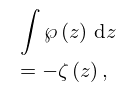
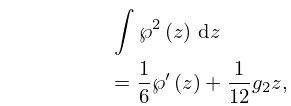
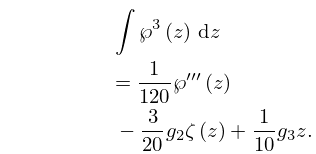
17: 23.14 Integrals

§23.14 Integrals

►

23.14.1 $$\int \mathrm{\wp }\left(z\right)dz=-\zeta \left(z\right),$$

ⓘ

Symbols:

$\mathrm{\wp }\left(z\right)$ (= $\mathrm{\wp }\left(z|𝕃\right)$ = $\mathrm{\wp }(z;g_2,g_3)$): Weierstrass $\mathrm{\wp }$-function, $\zeta \left(z\right)$ (= $\zeta \left(z|𝕃\right)$ = $\zeta (z;g_2,g_3)$): Weierstrass zeta function, $dx$: differential of $x$ , $\int$: integral, $𝕃$: lattice and $z$: complex

A&S Ref:

18.6.1

Permalink:

http://dlmf.nist.gov/23.14.E1

Encodings:

pMML, png, TeX

See also:

Annotations for §23.14 and Ch.23

►

23.14.2 $$\int {\mathrm{\wp }}^2\left(z\right)dz=\frac{1}{6}{\mathrm{\wp }}^{\prime }\left(z\right)+\frac{1}{12}{g}_{2}z,$$

ⓘ

Symbols:

$\mathrm{\wp }\left(z\right)$ (= $\mathrm{\wp }\left(z|𝕃\right)$ = $\mathrm{\wp }(z;g_2,g_3)$): Weierstrass $\mathrm{\wp }$-function, $g_j$: Weierstrass lattice invariants $g_2$, $g_3$ , $dx$: differential of $x$ , $\int$: integral, $𝕃$: lattice and $z$: complex

A&S Ref:

18.7.1

Permalink:

http://dlmf.nist.gov/23.14.E2

Encodings:

pMML, png, TeX

See also:

Annotations for §23.14 and Ch.23

►

23.14.3 $$\int {\mathrm{\wp }}^3\left(z\right)dz=\frac{1}{120}{\mathrm{\wp }}^{\prime \prime \prime }\left(z\right)-\frac{3}{20}{g}_2\zeta \left(z\right)+\frac{1}{10}{g}_{3}z.$$

ⓘ

Symbols:

$\mathrm{\wp }\left(z\right)$ (= $\mathrm{\wp }\left(z|𝕃\right)$ = $\mathrm{\wp }(z;g_2,g_3)$): Weierstrass $\mathrm{\wp }$-function, $g_j$: Weierstrass lattice invariants $g_2$, $g_3$ , $\zeta \left(z\right)$ (= $\zeta \left(z|𝕃\right)$ = $\zeta (z;g_2,g_3)$): Weierstrass zeta function, $dx$: differential of $x$ , $\int$: integral, $𝕃$: lattice and $z$: complex

A&S Ref:

18.7.2

Permalink:

http://dlmf.nist.gov/23.14.E3

Encodings:

pMML, png, TeX

See also:

Annotations for §23.14 and Ch.23

…

18: 19.2 Definitions

… ►Because $s^2$ is a polynomial, we have … ►

§19.2(ii) Legendre’s Integrals

… ►Legendre’s complementary complete elliptic integrals are defined via … ►

§19.2(iii) Bulirsch’s Integrals

►Bulirsch’s integrals are linear combinations of Legendre’s integrals that are chosen to facilitate computational application of Bartky’s transformation (Bartky (1938)). …

19: 23.13 Zeros

§23.13 Zeros

►For information on the zeros of $\mathrm{\wp }\left(z\right)$ see Eichler and Zagier (1982).

20: 23.10 Addition Theorems and Other Identities

… ►

§23.10(i) Addition Theorems

… ►

§23.10(ii) Duplication Formulas

… ►(23.10.8) continues to hold when $e_1$, $e_2$, $e_3$ are permuted cyclically. … ►

§23.10(iii) $n$-Tuple Formulas

… ►

§23.10(iv) Homogeneity

…