Weierstrass%20product

SearchAdvancedHelp

(0.002 seconds)

21—30 of 271 matching pages

21: 23.19 Interrelations

… ►

23.19.3 $$J\left(\tau \right)=\frac{g_2^3}{g_2^3-27g_3^2},$$

ⓘ

Symbols:

$J\left(\tau \right)$: Klein’s complete invariant, $g_j$: Weierstrass lattice invariants $g_2$, $g_3$ , $𝕃$: lattice and $\tau$: complex variable

Permalink:

http://dlmf.nist.gov/23.19.E3

Encodings:

pMML, png, TeX

See also:

Annotations for §23.19 and Ch.23

►where $g_2,g_3$ are the invariants of the lattice $𝕃$ with generators $1$ and $\tau$; see §23.3(i). …

22: 23.12 Asymptotic Approximations

§23.12 Asymptotic Approximations

… ►

23.12.1 $$\mathrm{\wp }\left(z\right)=\frac{{\pi }^2}{4{\omega }_1^2}\left(-\frac{1}{3}+{\csc }^2\left(\frac{\pi z}{2{\omega }_1}\right)+8\left(1-\cos \left(\frac{\pi z}{{\omega }_1}\right)\right)q^2+O\left(q^4\right)\right),$$

ⓘ

Symbols:

$O\left(x\right)$: order not exceeding, $\mathrm{\wp }\left(z\right)$ (= $\mathrm{\wp }\left(z|𝕃\right)$ = $\mathrm{\wp }(z;g_2,g_3)$): Weierstrass $\mathrm{\wp }$-function, $\pi$: the ratio of the circumference of a circle to its diameter, $\csc z$: cosecant function, $\cos z$: cosine function, $𝕃$: lattice, $q$: nome, $z$: complex and ${\omega }_1$, ${\omega }_3$, ${\omega }_2=-{\omega }_1-{\omega }_3$: lattice generators

Referenced by:

§23.12

Permalink:

http://dlmf.nist.gov/23.12.E1

Encodings:

pMML, png, TeX

See also:

Annotations for §23.12 and Ch.23

►

23.12.2 $$\zeta \left(z\right)=\frac{{\pi }^2}{4{\omega }_1^2}\left(\frac{z}{3}+\frac{2{\omega }_1}{\pi }\cot \left(\frac{\pi z}{2{\omega }_1}\right)-8\left(z-\frac{{\omega }_1}{\pi }\sin \left(\frac{\pi z}{{\omega }_1}\right)\right)q^2+O\left(q^4\right)\right),$$

ⓘ

Symbols:

$O\left(x\right)$: order not exceeding, $\zeta \left(z\right)$ (= $\zeta \left(z|𝕃\right)$ = $\zeta (z;g_2,g_3)$): Weierstrass zeta function, $\pi$: the ratio of the circumference of a circle to its diameter, $\cot z$: cotangent function, $\sin z$: sine function, $𝕃$: lattice, $q$: nome, $z$: complex and ${\omega }_1$, ${\omega }_3$, ${\omega }_2=-{\omega }_1-{\omega }_3$: lattice generators

Referenced by:

§23.12, Erratum (V1.0.23) for Equation (23.12.2)

Permalink:

http://dlmf.nist.gov/23.12.E2

Encodings:

pMML, png, TeX

Correction (effective with 1.0.23):

The factor of 2, previously omitted from the denominator of the argument of the $\cot$ function has been inserted.

Suggested 2019-05-27 by Blagoje Oblak

See also:

Annotations for §23.12 and Ch.23

►

23.12.3 $$\sigma \left(z\right)=\frac{2{\omega }_1}{\pi }\exp \left(\frac{{\pi }^2{z}^2}{24{\omega }_1^2}\right)\sin \left(\frac{\pi z}{2{\omega }_1}\right)\left(1-\left(\frac{{\pi }^2{z}^2}{{\omega }_1^2}-4{\sin }^2\left(\frac{\pi z}{2{\omega }_1}\right)\right)q^2+O\left(q^4\right)\right),$$

ⓘ

Symbols:

$O\left(x\right)$: order not exceeding, $\sigma \left(z\right)$ (= $\sigma \left(z|𝕃\right)$ = $\sigma (z;g_2,g_3)$): Weierstrass sigma function, $\pi$: the ratio of the circumference of a circle to its diameter, $\exp z$: exponential function, $\sin z$: sine function, $𝕃$: lattice, $q$: nome, $z$: complex and ${\omega }_1$, ${\omega }_3$, ${\omega }_2=-{\omega }_1-{\omega }_3$: lattice generators

Permalink:

http://dlmf.nist.gov/23.12.E3

Encodings:

pMML, png, TeX

See also:

Annotations for §23.12 and Ch.23

…

23: 31.2 Differential Equations

… ►

Weierstrass’s Form

… ►

$k^2=(e_2-e_3)/(e_1-e_3),$

… ►

$e_1=\mathrm{\wp }\left({\omega }_1\right),$

… ►

$e_1+e_2+e_3=0,$

►where $2{\omega }_1$ and $2{\omega }_3$ with $\mathrm{\Im }\left({\omega }_3/{\omega }_1\right)>0$ are generators of the lattice $𝕃$ for $\mathrm{\wp }\left(z|𝕃\right)$. …

24: 27.15 Chinese Remainder Theorem

… ►The Chinese remainder theorem states that a system of congruences $x\equiv a_1(mod{m}_1),\mathrm{\dots },x\equiv a_k(mod{m}_k)$, always has a solution if the moduli are relatively prime in pairs; the solution is unique (mod $m$), where $m$ is the product of the moduli. … ►Their product $m$ has 20 digits, twice the number of digits in the data. …These numbers, in turn, are combined by the Chinese remainder theorem to obtain the final result $(modm)$, which is correct to 20 digits. …

25: 1.10 Functions of a Complex Variable

… ►

§1.10(ix) Infinite Products

… ►The convergence of the infinite product is uniform if the sequence of partial products converges uniformly. ►

$M$-test

… ►

Weierstrass Product

…

26: 20 Theta Functions

Chapter 20 Theta Functions

…

27: 29.2 Differential Equations

… ►we have ►

29.2.9 $$\frac{d^{2}w}{{d\eta }^2}+(g-\nu (\nu +1)\mathrm{\wp }\left(\eta \right))w=0,$$

ⓘ

Symbols:

$\mathrm{\wp }\left(z\right)$ (= $\mathrm{\wp }\left(z|𝕃\right)$ = $\mathrm{\wp }(z;g_2,g_3)$): Weierstrass $\mathrm{\wp }$-function, $\frac{df}{dx}$: derivative of $f$ with respect to $x$ , $\nu$: real parameter, $g$ and $\eta$

Permalink:

http://dlmf.nist.gov/29.2.E9

Encodings:

pMML, png, TeX

See also:

Annotations for §29.2(ii), §29.2 and Ch.29

… ►

29.2.11 $$\zeta =\mathrm{\wp }(\eta ;g_2,g_3)=\mathrm{\wp }\left(\eta \right),$$

ⓘ

Defines:

$\zeta$ (locally)

Symbols:

$\mathrm{\wp }(z;g_2,g_3)$: Weierstrass $\mathrm{\wp }$-function, $\mathrm{\wp }\left(z\right)$ (= $\mathrm{\wp }\left(z|𝕃\right)$ = $\mathrm{\wp }(z;g_2,g_3)$): Weierstrass $\mathrm{\wp }$-function, $\eta$ , $g_2$ and $g_3$

Permalink:

http://dlmf.nist.gov/29.2.E11

Encodings:

pMML, png, TeX

See also:

Annotations for §29.2(ii), §29.2 and Ch.29

… ►For the Weierstrass function $\mathrm{\wp }$ see §23.2(ii). …

28: Errata

… ►

This subsection has been significantly updated. In particular, the following formulae have been corrected. Equation (19.25.35) has been replaced by

19.25.35 $$z+2\omega =\pm R_F(\mathrm{\wp }\left(z\right)-e_1,\mathrm{\wp }\left(z\right)-e_2,\mathrm{\wp }\left(z\right)-e_3),$$

in which the left-hand side $z$ has been replaced by $z+2\omega$ for some $2\omega \in 𝕃$, and the right-hand side has been multiplied by $\pm 1$. Equation (19.25.37) has been replaced by

19.25.37 $$\zeta \left(z+2\omega \right)+(z+2\omega )\mathrm{\wp }\left(z\right)=\pm 2R_G(\mathrm{\wp }\left(z\right)-e_1,\mathrm{\wp }\left(z\right)-e_2,\mathrm{\wp }\left(z\right)-e_3),$$

in which the left-hand side $\zeta \left(z\right)+z\mathrm{\wp }\left(z\right)$ has been replaced by $\zeta \left(z+2\omega \right)+(z+2\omega )\mathrm{\wp }\left(z\right)$ and the right-hand side has been multiplied by $\pm 1$. Equation (19.25.39) has been replaced by

19.25.39 $$\zeta \left({\omega }_j\right)+{\omega }_j{e}_j=2R_G(0,e_j-e_k,e_j-e_{\mathrm{\ell }}),$$

in which the left-hand side ${\eta }_j$ was replaced by $\zeta \left({\omega }_j\right)$, for some $2{\omega }_j\in 𝕃$ and $\mathrm{\wp }\left({\omega }_j\right)=e_j$. Equation (19.25.40) has been replaced by

19.25.40 $$z+2\omega =\pm \sigma \left(z\right)R_F({\sigma }_1^2(z),{\sigma }_2^2(z),{\sigma }_3^2(z)),$$

in which the left-hand side $z$ has been replaced by $z+2\omega$, and the right-hand side was multiplied by $\pm 1$. For more details see §19.25(vi).

… ►

The Weierstrass lattice roots $e_j,$ were linked inadvertently as the base of the natural logarithm. In order to resolve this inconsistency, the lattice roots $e_j$, and lattice invariants $g_2$, $g_3$, now link to their respective definitions (see §§23.2(i), 23.3(i)).

Reported by Felix Ospald.

►

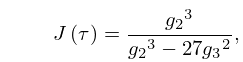
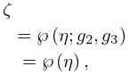
The Weierstrass zeta function was incorrectly linked to the definition of the Riemann zeta function. However, to the eye, the function appeared correct. The link was corrected.

… ►

23.2.4 $$\mathrm{\wp }\left(z\right)=\frac{1}{z^2}+\sum _{w\in 𝕃\setminus \{0\}}\left(\frac{1}{{(z-w)}^2}-\frac{1}{w^2}\right)$$

Originally the denominator ${(z-w)}^2$ was given incorrectly as $(z-w^2)$.

Reported 2012-02-16 by James D. Walker.

… ►

Several new equations have been added. See (8.17.24), (20.7.34), §20.11(v), (26.12.27), (36.2.28), and (36.2.29).

…

29: 26.12 Plane Partitions

… ►

26.12.9 $${\left(\prod _{h=1}^r\prod _{j=1}^s\frac{h+j+t-1}{h+j-1}\right)}^2;$$

ⓘ

Symbols:

$r$: positive integer, $s$: positive integer, $t$: positive integer, $h$: positive integer and $j$: positive integer

Permalink:

http://dlmf.nist.gov/26.12.E9

Encodings:

pMML, png, TeX

See also:

Annotations for §26.12(i), §26.12 and Ch.26

… ►

26.12.10 $$\left(\prod _{h=1}^r\prod _{j=1}^s\frac{h+j+t-1}{h+j-1}\right)\left(\prod _{h=1}^{r+1}\prod _{j=1}^s\frac{h+j+t-1}{h+j-1}\right);$$

ⓘ

Symbols:

$r$: positive integer, $s$: positive integer, $t$: positive integer, $h$: positive integer and $j$: positive integer

Permalink:

http://dlmf.nist.gov/26.12.E10

Encodings:

pMML, png, TeX

See also:

Annotations for §26.12(i), §26.12 and Ch.26

… ►

26.12.11 $$\left(\prod _{h=1}^{r+1}\prod _{j=1}^s\frac{h+j+t-1}{h+j-1}\right)\left(\prod _{h=1}^r\prod _{j=1}^{s+1}\frac{h+j+t-1}{h+j-1}\right).$$

ⓘ

Symbols:

$r$: positive integer, $s$: positive integer, $t$: positive integer, $h$: positive integer and $j$: positive integer

Permalink:

http://dlmf.nist.gov/26.12.E11

Encodings:

pMML, png, TeX

See also:

Annotations for §26.12(i), §26.12 and Ch.26

… ►

26.12.13 $$\prod _{h=1}^r\prod _{j=1}^r\frac{h+j+t-1}{h+j-1};$$

ⓘ

Symbols:

$r$: positive integer, $t$: positive integer, $h$: positive integer and $j$: positive integer

Permalink:

http://dlmf.nist.gov/26.12.E13

Encodings:

pMML, png, TeX

See also:

Annotations for §26.12(i), §26.12 and Ch.26

… ►

26.12.14 $$\prod _{h=1}^r\prod _{j=1}^{r+1}\frac{h+j+t-1}{h+j-1}.$$

ⓘ

Symbols:

$r$: positive integer, $t$: positive integer, $h$: positive integer and $j$: positive integer

Permalink:

http://dlmf.nist.gov/26.12.E14

Encodings:

pMML, png, TeX

See also:

Annotations for §26.12(i), §26.12 and Ch.26

…

30: Foreword

… ►The production of these new resources has been a very complex undertaking some 10 years in the making. … ►November 20, 2009 …