Weber–Schafheitlin discontinuous integrals

SearchAdvancedHelp

(0.002 seconds)

21—30 of 455 matching pages

21: 11.1 Special Notation

§11.1 Special Notation

… ►For the functions $J_{\nu }\left(z\right)$, $Y_{\nu }\left(z\right)$, $H_{\nu }^{(1)}\left(z\right)$, $H_{\nu }^{(2)}\left(z\right)$, $I_{\nu }\left(z\right)$, and $K_{\nu }\left(z\right)$ see §§10.2(ii), 10.25(ii). ►The functions treated in this chapter are the Struve functions ${𝐇}_{\nu }\left(z\right)$ and ${𝐊}_{\nu }\left(z\right)$, the modified Struve functions ${𝐋}_{\nu }\left(z\right)$ and ${𝐌}_{\nu }\left(z\right)$, the Lommel functions $s_{\mu ,\nu }\left(z\right)$ and $S_{\mu ,\nu }\left(z\right)$, the Anger function ${𝐉}_{\nu }\left(z\right)$, the Weber function ${𝐄}_{\nu }\left(z\right)$, and the associated Anger–Weber function ${𝐀}_{\nu }\left(z\right)$.

22: 10.1 Special Notation

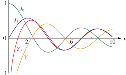
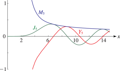
… ►The main functions treated in this chapter are the Bessel functions $J_{\nu }\left(z\right)$, $Y_{\nu }\left(z\right)$; Hankel functions $H_{\nu }^{(1)}\left(z\right)$, $H_{\nu }^{(2)}\left(z\right)$; modified Bessel functions $I_{\nu }\left(z\right)$, $K_{\nu }\left(z\right)$; spherical Bessel functions ${𝗃}_n\left(z\right)$, ${𝗒}_n\left(z\right)$, ${𝗁}_n^{(1)}\left(z\right)$, ${𝗁}_n^{(2)}\left(z\right)$; modified spherical Bessel functions ${𝗂}_n^{(1)}\left(z\right)$, ${𝗂}_n^{(2)}\left(z\right)$, ${𝗄}_n\left(z\right)$; Kelvin functions ${\mathrm{ber}}_{\nu }\left(x\right)$, ${\mathrm{bei}}_{\nu }\left(x\right)$, ${\ker }_{\nu }\left(x\right)$, ${\mathrm{kei}}_{\nu }\left(x\right)$. … ►A common alternative notation for $Y_{\nu }\left(z\right)$ is $N_{\nu }(z)$. … ►For older notations see British Association for the Advancement of Science (1937, pp. xix–xx) and Watson (1944, Chapters 1–3).

23: 10.24 Functions of Imaginary Order

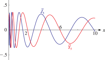
… ►and ${\tilde{J}}_{\nu }\left(x\right)$, ${\tilde{Y}}_{\nu }\left(x\right)$ are linearly independent solutions of (10.24.1): … ►In consequence of (10.24.6), when $x$ is large ${\tilde{J}}_{\nu }\left(x\right)$ and ${\tilde{Y}}_{\nu }\left(x\right)$ comprise a numerically satisfactory pair of solutions of (10.24.1); compare §2.7(iv). … ►For graphs of ${\tilde{J}}_{\nu }\left(x\right)$ and ${\tilde{Y}}_{\nu }\left(x\right)$ see §10.3(iii). ►For mathematical properties and applications of ${\tilde{J}}_{\nu }\left(x\right)$ and ${\tilde{Y}}_{\nu }\left(x\right)$, including zeros and uniform asymptotic expansions for large $\nu$, see Dunster (1990a). In this reference ${\tilde{J}}_{\nu }\left(x\right)$ and ${\tilde{Y}}_{\nu }\left(x\right)$ are denoted respectively by $F_{\mathrm{i}\nu }(x)$ and $G_{\mathrm{i}\nu }(x)$. …

24: 10.58 Zeros

… ►

$b_{n,m}=y_{n+\frac{1}{2},m},$

… ►

${𝗒}_n^{\prime }\left(b_{n,m}\right)=\sqrt{{\displaystyle \frac{\pi }{2y_{n+\frac{1}{2},m}}}}{Y}_{n+\frac{1}{2}}^{\prime }\left(y_{n+\frac{1}{2},m}\right).$

…

25: 10.74 Methods of Computation

… ►In the interval , $J_{\nu }\left(x\right)$ needs to be integrated in the forward direction and $Y_{\nu }\left(x\right)$ in the backward direction, with initial values for the former obtained from the power-series expansion (10.2.2) and for the latter from asymptotic expansions (§§10.17(i) and 10.20(i)). … ►Similarly, to maintain stability in the interval the integration direction has to be forwards in the case of $I_{\nu }\left(x\right)$ and backwards in the case of $K_{\nu }\left(x\right)$, with initial values obtained in an analogous manner to those for $J_{\nu }\left(x\right)$ and $Y_{\nu }\left(x\right)$. … ►

§10.74(iii) Integral Representations

… ►If values of the Bessel functions $J_{\nu }\left(z\right)$, $Y_{\nu }\left(z\right)$, or the other functions treated in this chapter, are needed for integer-spaced ranges of values of the order $\nu$, then a simple and powerful procedure is provided by recurrence relations typified by the first of (10.6.1). … ►Then $J_n\left(x\right)$ and $Y_n\left(x\right)$ can be generated by either forward or backward recurrence on $n$ when , but if $n>x$ then to maintain stability $J_n\left(x\right)$ has to be generated by backward recurrence on $n$, and $Y_n\left(x\right)$ has to be generated by forward recurrence on $n$. …

26: 10.3 Graphics

… ►

►►

Figure 10.3.1: $J_0\left(x\right)$, $Y_0\left(x\right)$, $J_1\left(x\right)$, $Y_1\left(x\right)$, $0\le x\le 10$. Magnify

►

►►

Figure 10.3.2: $J_5\left(x\right)$, $Y_5\left(x\right)$, $M_5\left(x\right)$, $0\le x\le 15$. Magnify

… ►

►►

Figure 10.3.17: ${\tilde{J}}_{1/2}\left(x\right)$, ${\tilde{Y}}_{1/2}\left(x\right)$, $0.01\le x\le 10$. Magnify

►

►►

Figure 10.3.18: ${\tilde{J}}_1\left(x\right)$, ${\tilde{Y}}_1\left(x\right)$, $0.01\le x\le 10$. Magnify

►

►►

Figure 10.3.19: ${\tilde{J}}_5\left(x\right)$, ${\tilde{Y}}_5\left(x\right)$, $0.01\le x\le 10$. Magnify

27: 10.4 Connection Formulas

… ►Other solutions of (10.2.1) include $J_{-\nu }\left(z\right)$, $Y_{-\nu }\left(z\right)$, $H_{-\nu }^{(1)}\left(z\right)$, and $H_{-\nu }^{(2)}\left(z\right)$. … ►

$$Y_{-n}\left(z\right)={(-1)}^n{Y}_n\left(z\right),$$

… ►

$$H_{\nu }^{(1)}\left(z\right)=J_{\nu }\left(z\right)+\mathrm{i}{Y}_{\nu }\left(z\right),$$

►

$$H_{\nu }^{(2)}\left(z\right)=J_{\nu }\left(z\right)-\mathrm{i}{Y}_{\nu }\left(z\right),$$

… ►

10.4.5 $$J_{\nu }\left(z\right)=\csc \left(\nu \pi \right)\left(Y_{-\nu }\left(z\right)-Y_{\nu }\left(z\right)\cos \left(\nu \pi \right)\right).$$

ⓘ

Symbols:

$J_{\nu }\left(z\right)$: Bessel function of the first kind, $Y_{\nu }\left(z\right)$: Bessel function of the second kind, $\pi$: the ratio of the circumference of a circle to its diameter, $\csc z$: cosecant function, $\cos z$: cosine function, $z$: complex variable and $\nu$: complex parameter

Referenced by:

§10.4

Permalink:

http://dlmf.nist.gov/10.4.E5

Encodings:

pMML, png, TeX

See also:

Annotations for §10.4 and Ch.10

…

28: 12.1 Special Notation

… ►Unless otherwise noted, primes indicate derivatives with respect to the variable, and fractional powers take their principal values. ►The main functions treated in this chapter are the parabolic cylinder functions (PCFs), also known as Weber parabolic cylinder functions: $U(a,z)$, $V(a,z)$, $\overline{U}(a,z)$, and $W(a,z)$. …

29: 10.9 Integral Representations

§10.9 Integral Representations

… ►

Bessel’s Integral

… ►

§10.9(ii) Contour Integrals

… ►

Hankel’s Integrals

… ► …

30: 3.6 Linear Difference Equations

… ►is satisfied by $J_n\left(1\right)$ and $Y_n\left(1\right)$, where $J_n\left(x\right)$ and $Y_n\left(x\right)$ are the Bessel functions of the first kind. … ►

Example 2. Weber Function

►The Weber function ${𝐄}_n\left(1\right)$ satisfies …Thus the asymptotic behavior of the particular solution ${𝐄}_n\left(1\right)$ is intermediate to those of the complementary functions $J_n\left(1\right)$ and $Y_n\left(1\right)$; moreover, the conditions for Olver’s algorithm are satisfied. We apply the algorithm to compute ${𝐄}_n\left(1\right)$ to 8S for the range $n=1,2,\mathrm{\dots },10$, beginning with the value ${𝐄}_0\left(1\right)=-\mathrm{0.56865\hspace{0.33em}\hspace{0.17em}663}$ obtained from the Maclaurin series expansion (§11.10(iii)). …