Narayana numbers

SearchAdvancedHelp

(0.001 seconds)

41—50 of 223 matching pages

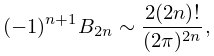
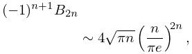
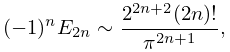
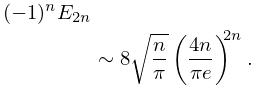
41: 24.11 Asymptotic Approximations

§24.11 Asymptotic Approximations

… ►

24.11.1 $${(-1)}^{n+1}{B}_{2n}\sim \frac{2(2n)!}{{(2\pi )}^{2n}},$$

ⓘ

Symbols:

$B_n$: Bernoulli numbers, $\sim$: asymptotic equality, $\pi$: the ratio of the circumference of a circle to its diameter, $!$: factorial (as in $n!$) and $n$: integer

Referenced by:

§24.11

Permalink:

http://dlmf.nist.gov/24.11.E1

Encodings:

pMML, png, TeX

See also:

Annotations for §24.11 and Ch.24

►

24.11.2 $${(-1)}^{n+1}{B}_{2n}\sim 4\sqrt{\pi n}{\left(\frac{n}{\pi \mathrm{e}}\right)}^{2n},$$

ⓘ

Symbols:

$B_n$: Bernoulli numbers, $\sim$: asymptotic equality, $\pi$: the ratio of the circumference of a circle to its diameter, $\mathrm{e}$: base of natural logarithm and $n$: integer

Permalink:

http://dlmf.nist.gov/24.11.E2

Encodings:

pMML, png, TeX

See also:

Annotations for §24.11 and Ch.24

►

24.11.3 $${(-1)}^n{E}_{2n}\sim \frac{2^{2n+2}(2n)!}{{\pi }^{2n+1}},$$

ⓘ

Symbols:

$E_n$: Euler numbers, $\sim$: asymptotic equality, $\pi$: the ratio of the circumference of a circle to its diameter, $!$: factorial (as in $n!$) and $n$: integer

Permalink:

http://dlmf.nist.gov/24.11.E3

Encodings:

pMML, png, TeX

See also:

Annotations for §24.11 and Ch.24

►

24.11.4 $${(-1)}^n{E}_{2n}\sim 8\sqrt{\frac{n}{\pi }}{\left(\frac{4n}{\pi \mathrm{e}}\right)}^{2n}.$$

ⓘ

Symbols:

$E_n$: Euler numbers, $\sim$: asymptotic equality, $\pi$: the ratio of the circumference of a circle to its diameter, $\mathrm{e}$: base of natural logarithm and $n$: integer

Referenced by:

§24.11

Permalink:

http://dlmf.nist.gov/24.11.E4

Encodings:

pMML, png, TeX

See also:

Annotations for §24.11 and Ch.24

…

42: 27.5 Inversion Formulas

§27.5 Inversion Formulas

… ►Generating functions yield many relations connecting number-theoretic functions. … ►Special cases of Möbius inversion pairs are: … ►Other types of Möbius inversion formulas include: … ►

43: 27.20 Methods of Computation: Other Number-Theoretic Functions

§27.20 Methods of Computation: Other Number-Theoretic Functions

…

44: 24.16 Generalizations

§24.16 Generalizations

… ►

Polynomials and Numbers of Integer Order

… ►

Bernoulli Numbers of the Second Kind

… ►

Degenerate Bernoulli Numbers

… ►

§24.16(iii) Other Generalizations

…

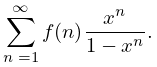
45: 27.7 Lambert Series as Generating Functions

§27.7 Lambert Series as Generating Functions

►Lambert series have the form ►

27.7.1 $$\sum _{n=1}^{\mathrm{\infty }}f(n)\frac{x^n}{1-x^n}.$$

ⓘ

Symbols:

$n$: positive integer and $x$: real number

Referenced by:

§27.7

Permalink:

http://dlmf.nist.gov/27.7.E1

Encodings:

pMML, png, TeX

See also:

Annotations for §27.7 and Ch.27

… ►

27.7.3 $$\sum _{n=1}^{\mathrm{\infty }}\mu \left(n\right)\frac{x^n}{1-x^n}=x,$$

ⓘ

Symbols:

$\mu \left(n\right)$: Möbius function, $n$: positive integer and $x$: real number

A&S Ref:

24.3.1 I.B

Permalink:

http://dlmf.nist.gov/27.7.E3

Encodings:

pMML, png, TeX

See also:

Annotations for §27.7 and Ch.27

… ►

27.7.5 $$\sum _{n=1}^{\mathrm{\infty }}{n}^{\alpha }\frac{x^n}{1-x^n}=\sum _{n=1}^{\mathrm{\infty }}{\sigma }_{\alpha }\left(n\right)x^n,$$

ⓘ

Symbols:

${\sigma }_{\alpha }\left(n\right)$: sum of powers of divisors of a number, $n$: positive integer and $x$: real number

A&S Ref:

24.3.3 I.B

Permalink:

http://dlmf.nist.gov/27.7.E5

Encodings:

pMML, png, TeX

See also:

Annotations for §27.7 and Ch.27

…

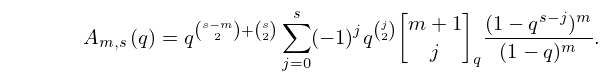
46: 17.3 $q$-Elementary and $q$-Special Functions

… ►

§17.3(iii) Bernoulli Polynomials; Euler and Stirling Numbers

… ►

$q$-Euler Numbers

►

17.3.8 $$A_{m,s}\left(q\right)=q^{\left(\genfrac{}{}{0.0pt}{}{s-m}{2}\right)+\left(\genfrac{}{}{0.0pt}{}{s}{2}\right)}\sum _{j=0}^s{(-1)}^j{q}^{\left(\genfrac{}{}{0.0pt}{}{j}{2}\right)}{\left[\genfrac{}{}{0.0pt}{}{m+1}{j}\right]}_q\frac{{(1-q^{s-j})}^m}{{(1-q)}^m}.$$

ⓘ

Defines:

$A_{m,s}\left(q\right)$: $q$-Euler number

Symbols:

$\left(\genfrac{}{}{0.0pt}{}{m}{n}\right)$: binomial coefficient, ${\left[\genfrac{}{}{0.0pt}{}{n}{m}\right]}_q$: $q$-binomial coefficient (or Gaussian polynomial), $q$: complex base, $j$: nonnegative integer, $m$: nonnegative integer and $s$: nonnegative integer

Permalink:

http://dlmf.nist.gov/17.3.E8

Encodings:

pMML, png, TeX

See also:

Annotations for §17.3(iii), §17.3(iii), §17.3 and Ch.17

►

$q$-Stirling Numbers

… ►The $A_{m,s}\left(q\right)$ are always polynomials in $q$, and the $a_{m,s}\left(q\right)$ are polynomials in $q$ for $0\le s\le m$. …

47: 20.12 Mathematical Applications

… ►

§20.12(i) Number Theory

… ►For applications of Jacobi’s triple product (20.5.9) to Ramanujan’s $\tau \left(n\right)$ function and Euler’s pentagonal numbers see Hardy and Wright (1979, pp. 132–160) and McKean and Moll (1999, pp. 143–145). … ►The space of complex tori $ℂ/(\mathbb{Z}+\tau \mathbb{Z})$ (that is, the set of complex numbers $z$ in which two of these numbers $z_1$ and $z_2$ are regarded as equivalent if there exist integers $m,n$ such that $z_1-z_2=m+\tau n$) is mapped into the projective space $P^3$ via the identification $z\to ({\theta }_1\left(2z\right|\tau ),{\theta }_2\left(2z\right|\tau ),{\theta }_3\left(2z\right|\tau ),{\theta }_4\left(2z\right|\tau ))$. …

48: 27.11 Asymptotic Formulas: Partial Sums

§27.11 Asymptotic Formulas: Partial Sums

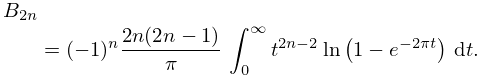
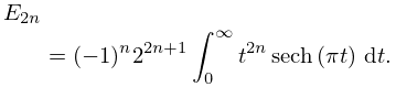
►The behavior of a number-theoretic function $f(n)$ for large $n$ is often difficult to determine because the function values can fluctuate considerably as $n$ increases. … ►where $\left(h,k\right)=1$, $k>0$. … ►Each of (27.11.13)–(27.11.15) is equivalent to the prime number theorem (27.2.3). The prime number theorem for arithmetic progressions—an extension of (27.2.3) and first proved in de la Vallée Poussin (1896a, b)—states that if $\left(h,k\right)=1$, then the number of primes $p\le x$ with $p\equiv h(modk)$ is asymptotic to $x/(\varphi \left(k\right)\ln x)$ as $x\to \mathrm{\infty }$.

49: 24.7 Integral Representations

… ►

§24.7(i) Bernoulli and Euler Numbers

… ►

24.7.3 $$B_{2n}={(-1)}^{n+1}\frac{\pi }{1-2^{1-2n}}{\int }_0^{\mathrm{\infty }}{t}^{2n}{\mathrm{sech}}^2\left(\pi t\right)dt,$$

ⓘ

Symbols:

$B_n$: Bernoulli numbers, $\pi$: the ratio of the circumference of a circle to its diameter, $dx$: differential of $x$ , $\mathrm{sech}z$: hyperbolic secant function, $\int$: integral, $n$: integer and $t$: real or complex

Permalink:

http://dlmf.nist.gov/24.7.E3

Encodings:

pMML, png, TeX

See also:

Annotations for §24.7(i), §24.7 and Ch.24

►

24.7.4 $$B_{2n}={(-1)}^{n+1}\pi {\int }_0^{\mathrm{\infty }}{t}^{2n}{\mathrm{csch}}^2\left(\pi t\right)dt,$$

ⓘ

Symbols:

$B_n$: Bernoulli numbers, $\pi$: the ratio of the circumference of a circle to its diameter, $dx$: differential of $x$ , $\mathrm{csch}z$: hyperbolic cosecant function, $\int$: integral, $n$: integer and $t$: real or complex

Permalink:

http://dlmf.nist.gov/24.7.E4

Encodings:

pMML, png, TeX

See also:

Annotations for §24.7(i), §24.7 and Ch.24

►

24.7.5 $$B_{2n}={(-1)}^n\frac{2n(2n-1)}{\pi }{\int }_0^{\mathrm{\infty }}{t}^{2n-2}\ln \left(1-{\mathrm{e}}^{-2\pi t}\right)dt.$$

ⓘ

Symbols:

$B_n$: Bernoulli numbers, $\pi$: the ratio of the circumference of a circle to its diameter, $dx$: differential of $x$ , $\mathrm{e}$: base of natural logarithm, $\int$: integral, $\ln z$: principal branch of logarithm function, $n$: integer and $t$: real or complex

Referenced by:

§24.7(i)

Permalink:

http://dlmf.nist.gov/24.7.E5

Encodings:

pMML, png, TeX

See also:

Annotations for §24.7(i), §24.7 and Ch.24

►

24.7.6 $$E_{2n}={(-1)}^n{2}^{2n+1}{\int }_0^{\mathrm{\infty }}{t}^{2n}\mathrm{sech}\left(\pi t\right)dt.$$

ⓘ

Symbols:

$E_n$: Euler numbers, $\pi$: the ratio of the circumference of a circle to its diameter, $dx$: differential of $x$ , $\mathrm{sech}z$: hyperbolic secant function, $\int$: integral, $n$: integer and $t$: real or complex

Referenced by:

§24.7(i)

Permalink:

http://dlmf.nist.gov/24.7.E6

Encodings:

pMML, png, TeX

See also:

Annotations for §24.7(i), §24.7 and Ch.24

…

50: 19.38 Approximations

… ►The accuracy is controlled by the number of terms retained in the approximation; for real variables the number of significant figures appears to be roughly twice the number of terms retained, perhaps even for $\varphi$ near $\pi /2$ with the improvements made in the 1970 reference. …