Legendre%0Aelliptic%20integrals

SearchAdvancedHelp

(0.003 seconds)

11—20 of 807 matching pages

11: 36.2 Catastrophes and Canonical Integrals

… ►

Canonical Integrals

… ►with the contour passing to the lower right of $u=0$. …with the contour passing to the upper right of $u=0$. … ► … ►

§36.2(iii) Symmetries

…

12: 27.9 Quadratic Characters

§27.9 Quadratic Characters

►For an odd prime $p$, the Legendre symbol $(n|p)$ is defined as follows. If $p$ divides $n$, then the value of $(n|p)$ is $0$. If $p$ does not divide $n$, then $(n|p)$ has the value $1$ when the quadratic congruence $x^2\equiv n(modp)$ has a solution, and the value $-1$ when this congruence has no solution. The Legendre symbol $(n|p)$, as a function of $n$, is a Dirichlet character (mod $p$). …

13: 14.21 Definitions and Basic Properties

… ►

§14.21(i) Associated Legendre Equation

… ► ►

§14.21(ii) Numerically Satisfactory Solutions

►When $\mathrm{\Re }\nu \ge -\frac{1}{2}$ and $\mathrm{\Re }\mu \ge 0$, a numerically satisfactory pair of solutions of (14.21.1) in the half-plane $|\mathrm{ph}z|\le \frac{1}{2}\pi$ is given by $P_{\nu }^{-\mu }\left(z\right)$ and ${𝑸}_{\nu }^{\mu }\left(z\right)$. ►

§14.21(iii) Properties

…

14: 14.6 Integer Order

§14.6 Integer Order

… ►For $m=0,1,2,\mathrm{\dots }$, … ►

14.6.6 $${𝖯}_{\nu }^{-m}\left(x\right)={\left(1-x^2\right)}^{-m/2}{\int }_x^1\mathrm{\dots }{\int }_x^1{𝖯}_{\nu }\left(x\right){\left(dx\right)}^m.$$

ⓘ

Symbols:

: Ferrers function of the first kind, $dx$: differential of $x$ , $\int$: integral, ${𝖯}_{\nu }\left(x\right)={𝖯}_{\nu }^0\left(x\right)$: Ferrers function of the first kind, $P_{\nu }\left(z\right)=P_{\nu }^0\left(z\right)$: Legendre function of the first kind, $x$: real variable, $m$: nonnegative integer and $\nu$: general degree

Referenced by:

§14.12(i), Erratum (V1.0.28) for Equation (14.6.6)

Permalink:

http://dlmf.nist.gov/14.6.E6

Encodings:

pMML, png, TeX

Clarification (effective with 1.0.28):

The right-hand side has been corrected by replacing the Legendre function $P_{\nu }\left(x\right)$ with the Ferrers function ${𝖯}_{\nu }\left(x\right)$.

See also:

Annotations for §14.6(ii), §14.6 and Ch.14

►

14.6.7 $$P_{\nu }^{-m}\left(x\right)={\left(x^2-1\right)}^{-m/2}{\int }_1^x\mathrm{\dots }{\int }_1^x{P}_{\nu }\left(x\right){\left(dx\right)}^m,$$

ⓘ

Symbols:

$P_{\nu }^{\mu }\left(z\right)$: associated Legendre function of the first kind, $dx$: differential of $x$ , $\int$: integral, $P_{\nu }\left(z\right)=P_{\nu }^0\left(z\right)$: Legendre function of the first kind, $x$: real variable, $m$: nonnegative integer and $\nu$: general degree

A&S Ref:

8.14.17

Referenced by:

§14.21(iii)

Permalink:

http://dlmf.nist.gov/14.6.E7

Encodings:

pMML, png, TeX

See also:

Annotations for §14.6(ii), §14.6 and Ch.14

… ►

15: 14.4 Graphics

… ►

§14.4(iii) Associated Legendre Functions: 2D Graphs

… ►

►►

Figure 14.4.24: ${𝑸}_0^{\mu }\left(x\right)$, $\mu =0,2,4,8$. Magnify

… ►

►►

Figure 14.4.28: ${𝑸}_1^{\mu }\left(x\right)$, $\mu =0,2,4,8$. Magnify

►

§14.4(iv) Associated Legendre Functions: 3D Surfaces

… ►

►

►

Figure 14.4.32: ${𝑸}_0^{\mu }\left(x\right)$, $0\le \mu \le 10$, . Magnify 3D Help

16: 14.7 Integer Degree and Order

… ►

§14.7(i) $\mu =0$

… ►where $P_n\left(x\right)$ is the Legendre polynomial of degree $n$. … ►

§14.7(ii) Rodrigues-Type Formulas

… ►

§14.7(iv) Generating Functions

… ►

17: 14.5 Special Values

… ►

§14.5(i) $x=0$

… ►

§14.5(ii) $\mu =0$, $\nu =0,1$

… ►In this subsection and the next two, and $\xi >0$. … ►

§14.5(v) $\mu =0$, $\nu =\pm \frac{1}{2}$

… ► …

18: 14.18 Sums

§14.18 Sums

… ► … ►In these formulas the Legendre functions are as in §14.3(ii) with $\mu =0$. … ►

Dougall’s Expansion

… ►

19: 14.2 Differential Equations

… ►

§14.2(i) Legendre’s Equation

… ►

§14.2(ii) Associated Legendre Equation

… ►Ferrers functions and the associated Legendre functions are related to the Legendre functions by the equations ${𝖯}_{\nu }^0\left(x\right)={𝖯}_{\nu }\left(x\right)$, ${𝖰}_{\nu }^0\left(x\right)={𝖰}_{\nu }\left(x\right)$, $P_{\nu }^0\left(x\right)=P_{\nu }\left(x\right)$, $Q_{\nu }^0\left(x\right)=Q_{\nu }\left(x\right)$, ${𝑸}_{\nu }^0\left(x\right)={𝑸}_{\nu }\left(x\right)=Q_{\nu }\left(x\right)/\mathrm{\Gamma }\left(\nu +1\right)$. … ►

§14.2(iii) Numerically Satisfactory Solutions

… ►When $\mathrm{\Re }\mu \ge 0$ and $\mathrm{\Re }\nu \ge -\frac{1}{2}$, $P_{\nu }^{-\mu }\left(x\right)$ and ${𝑸}_{\nu }^{\mu }\left(x\right)$ are linearly independent, and recessive at $x=1$ and $x=\mathrm{\infty }$, respectively. …

20: 14.33 Tables

§14.33 Tables

►

Abramowitz and Stegun (1964, Chapter 8) tabulates ${𝖯}_n\left(x\right)$ for $n=0(1)3,9,10$, $x=0(.01)1$, 5–8D; ${𝖯}_n^{\prime }\left(x\right)$ for $n=1(1)4,9,10$, $x=0(.01)1$, 5–7D; ${𝖰}_n\left(x\right)$ and ${𝖰}_n^{\prime }\left(x\right)$ for $n=0(1)3,9,10$, $x=0(.01)1$, 6–8D; $P_n\left(x\right)$ and $P_n^{\prime }\left(x\right)$ for $n=0(1)5,9,10$, $x=1(.2)10$, 6S; $Q_n\left(x\right)$ and $Q_n^{\prime }\left(x\right)$ for $n=0(1)3,9,10$, $x=1(.2)10$, 6S. (Here primes denote derivatives with respect to $x$.)

►

Zhang and Jin (1996, Chapter 4) tabulates ${𝖯}_n\left(x\right)$ for $n=2(1)5,10$, $x=0(.1)1$, 7D; ${𝖯}_n\left(\cos \theta \right)$ for $n=1(1)4,10$, $\theta =0(5^{\circ }){90}^{\circ }$, 8D; ${𝖰}_n\left(x\right)$ for $n=0(1)2,10$, $x=0(.1)0.9$, 8S; ${𝖰}_n\left(\cos \theta \right)$ for $n=0(1)3,10$, $\theta =0(5^{\circ }){90}^{\circ }$, 8D; ${𝖯}_n^m\left(x\right)$ for $m=1(1)4$, $n-m=0(1)2$, $n=10$, $x=0,0.5$, 8S; ${𝖰}_n^m\left(x\right)$ for $m=1(1)4$, $n=0(1)2,10$, 8S; ${𝖯}_{\nu }^m\left(\cos \theta \right)$ for $m=0(1)3$, $\nu =0(.25)5$, $\theta =0({15}^{\circ }){90}^{\circ }$, 5D; $P_n\left(x\right)$ for $n=2(1)5,10$, $x=1(1)10$, 7S; $Q_n\left(x\right)$ for $n=0(1)2,10$, $x=2(1)10$, 8S. Corresponding values of the derivative of each function are also included, as are 6D values of the first 5 $\nu$-zeros of ${𝖯}_{\nu }^m\left(\cos \theta \right)$ and of its derivative for $m=0(1)4$, $\theta ={10}^{\circ },{30}^{\circ },{150}^{\circ }$.

►

Belousov (1962) tabulates ${𝖯}_n^m\left(\cos \theta \right)$ (normalized) for $m=0(1)36$, $n-m=0(1)56$, $\theta =0({2.5}^{\circ }){90}^{\circ }$, 6D.

►

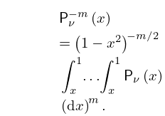
Žurina and Karmazina (1964, 1965) tabulate the conical functions ${𝖯}_{-\frac{1}{2}+\mathrm{i}\tau }\left(x\right)$ for $\tau =0(.01)50$, $x=-0.9(.1)0.9$, 7S; $P_{-\frac{1}{2}+\mathrm{i}\tau }\left(x\right)$ for $\tau =0(.01)50$, $x=1.1(.1)2(.2)5(.5)10(10)60$, 7D. Auxiliary tables are included to facilitate computation for larger values of $\tau$ when .

…