Lauricella%0Afunction

SearchAdvancedHelp

(0.002 seconds)

21—30 of 699 matching pages

21: 20.15 Tables

… ►This reference gives ${\theta }_j(x,q)$, $j=1,2,3,4$, and their logarithmic $x$-derivatives to 4D for $x/\pi =0(.1)1$, $\alpha =0(9^{\circ }){90}^{\circ }$, where $\alpha$ is the modular angle given by ►

20.15.1 $$\sin \alpha ={\theta }_2^2(0,q)/{\theta }_3^2(0,q)=k.$$

ⓘ

Defines:

$\alpha$: modular angle (locally)

Symbols:

${\theta }_j(z,q)$: theta function, $\sin z$: sine function and $q$: nome

Referenced by:

§20.15, §20.15

Permalink:

http://dlmf.nist.gov/20.15.E1

Encodings:

pMML, png, TeX

See also:

Annotations for §20.15 and Ch.20

►Spenceley and Spenceley (1947) tabulates ${\theta }_1(x,q)/{\theta }_2(0,q)$, ${\theta }_2(x,q)/{\theta }_2(0,q)$, ${\theta }_3(x,q)/{\theta }_4(0,q)$, ${\theta }_4(x,q)/{\theta }_4(0,q)$ to 12D for $u=0(1^{\circ }){90}^{\circ }$, $\alpha =0(1^{\circ }){89}^{\circ }$, where $u=2x/(\pi {\theta }_3^2(0,q))$ and $\alpha$ is defined by (20.15.1), together with the corresponding values of ${\theta }_2(0,q)$ and ${\theta }_4(0,q)$. ►Lawden (1989, pp. 270–279) tabulates ${\theta }_j(x,q)$, $j=1,2,3,4$, to 5D for $x=0(1^{\circ }){90}^{\circ }$, $q=0.1(.1)0.9$, and also $q$ to 5D for $k^2=0(.01)1$. ►Tables of Neville’s theta functions ${\theta }_s(x,q)$, ${\theta }_c(x,q)$, ${\theta }_d(x,q)$, ${\theta }_n(x,q)$ (see §20.1) and their logarithmic $x$-derivatives are given in Abramowitz and Stegun (1964, pp. 582–585) to 9D for $\epsilon ,\alpha =0(5^{\circ }){90}^{\circ }$, where (in radian measure) $\epsilon =x/{\theta }_3^2(0,q)=\pi x/(2K\left(k\right))$, and $\alpha$ is defined by (20.15.1). …

22: 10.72 Mathematical Applications

… ►These expansions are uniform with respect to $z$, including the turning point $z_0$ and its neighborhood, and the region of validity often includes cut neighborhoods (§1.10(vi)) of other singularities of the differential equation, especially irregular singularities. … ►The number $m$ can also be replaced by any real constant $\lambda$ $(>-2)$ in the sense that ${(z-z_0)}^{-\lambda }$ $f(z)$ is analytic and nonvanishing at $z_0$; moreover, $g(z)$ is permitted to have a single or double pole at $z_0$. … ►In regions in which the function $f(z)$ has a simple pole at $z=z_0$ and ${(z-z_0)}^{2}g(z)$ is analytic at $z=z_0$ (the case $\lambda =-1$ in §10.72(i)), asymptotic expansions of the solutions $w$ of (10.72.1) for large $u$ can be constructed in terms of Bessel functions and modified Bessel functions of order $\pm \sqrt{1+4\rho }$, where $\rho$ is the limiting value of ${(z-z_0)}^{2}g(z)$ as $z\to z_0$. … ►In (10.72.1) assume $f(z)=f(z,\alpha )$ and $g(z)=g(z,\alpha )$ depend continuously on a real parameter $\alpha$, $f(z,\alpha )$ has a simple zero $z=z_0(\alpha )$ and a double pole $z=0$, except for a critical value $\alpha =a$, where $z_0(a)=0$. …These approximations are uniform with respect to both $z$ and $\alpha$, including $z=z_0(a)$, the cut neighborhood of $z=0$, and $\alpha =a$. …

23: 28.21 Graphics

… ►

►

►

Figure 28.21.1: ${\mathrm{Mc}}_0^{(1)}(x,h)$ for $0\le h\le 3$, $0\le x\le 2$. Magnify 3D Help

►

►

►

Figure 28.21.2: ${\mathrm{Mc}}_1^{(1)}(x,h)$ for $0\le h\le 3$, $0\le x\le 2$. Magnify 3D Help

►

►

►

Figure 28.21.3: ${\mathrm{Mc}}_0^{(2)}(x,h)$ for $0.1\le h\le 2$, $0\le x\le 2$. Magnify 3D Help

►

►

►

Figure 28.21.4: ${\mathrm{Mc}}_1^{(2)}(x,h)$ for $0.2\le h\le 2$, $0\le x\le 2$. Magnify 3D Help

►

►

►

Figure 28.21.5: ${\mathrm{Ms}}_1^{(1)}(x,h)$ for $0\le h\le 3$, $0\le x\le 2$. Magnify 3D Help

…

24: 28.35 Tables

… ►

Blanch and Clemm (1962) includes values of ${\mathrm{Mc}}_n^{(1)}(x,\sqrt{q})$ and $\mathrm{Mc}_n^{(1)}{}_{}{}^{\prime }(x,\sqrt{q})$ for $n=0(1)15$ with $q=0(.05)1$, $x=0(.02)1$. Also ${\mathrm{Ms}}_n^{(1)}(x,\sqrt{q})$ and $\mathrm{Ms}_n^{(1)}{}_{}{}^{\prime }(x,\sqrt{q})$ for $n=1(1)15$ with $q=0(.05)1$, $x=0(.02)1$. Precision is generally 7D.

►

Blanch and Clemm (1965) includes values of ${\mathrm{Mc}}_n^{(2)}(x,\sqrt{q})$, $\mathrm{Mc}_n^{(2)}{}_{}{}^{\prime }(x,\sqrt{q})$ for $n=0(1)7$, $x=0(.02)1$; $n=8(1)15$, $x=0(.01)1$. Also ${\mathrm{Ms}}_n^{(2)}(x,\sqrt{q})$, $\mathrm{Ms}_n^{(2)}{}_{}{}^{\prime }(x,\sqrt{q})$ for $n=1(1)7$, $x=0(.02)1$; $n=8(1)15$, $x=0(.01)1$. In all cases $q=0(.05)1$. Precision is generally 7D. Approximate formulas and graphs are also included.

… ►

National Bureau of Standards (1967) includes the eigenvalues $a_n\left(q\right)$, $b_n\left(q\right)$ for $n=0(1)3$ with $q=0(.2)20(.5)37(1)100$, and $n=4(1)15$ with $q=0(2)100$; Fourier coefficients for ${\mathrm{ce}}_n(x,q)$ and ${\mathrm{se}}_n(x,q)$ for $n=0(1)15$, $n=1(1)15$, respectively, and various values of $q$ in the interval $[0,100]$; joining factors $g_{e,n}(\sqrt{q})$, $f_{e,n}(\sqrt{q})$ for $n=0(1)15$ with $q=0(.5\text{ to }10)100$ (but in a different notation). Also, eigenvalues for large values of $q$. Precision is generally 8D.

… ►

Zhang and Jin (1996, pp. 521–532) includes the eigenvalues $a_n\left(q\right)$, $b_{n+1}\left(q\right)$ for $n=0(1)4$, $q=0(1)50$; $n=0(1)20$ ($a$’s) or 19 ($b$’s), $q=1,3,5,10,15,25,50(50)200$. Fourier coefficients for ${\mathrm{ce}}_n(x,10)$, ${\mathrm{se}}_{n+1}(x,10)$, $n=0(1)7$. Mathieu functions ${\mathrm{ce}}_n(x,10)$, ${\mathrm{se}}_{n+1}(x,10)$, and their first $x$-derivatives for $n=0(1)4$, $x=0(5^{\circ }){90}^{\circ }$. Modified Mathieu functions ${\mathrm{Mc}}_n^{(j)}(x,\sqrt{10})$, ${\mathrm{Ms}}_{n+1}^{(j)}(x,\sqrt{10})$, and their first $x$-derivatives for $n=0(1)4$, $j=1,2$, $x=0(.2)4$. Precision is mostly 9S.

… ►

Blanch and Clemm (1969) includes eigenvalues $a_n\left(q\right)$, $b_n\left(q\right)$ for $q=\rho {\mathrm{e}}^{\mathrm{i}\varphi }$, $\rho =0(.5)25$, $\varphi =5^{\circ }(5^{\circ }){90}^{\circ }$, $n=0(1)15$; 4D. Also $a_n\left(q\right)$ and $b_n\left(q\right)$ for $q=\mathrm{i}\rho$, $\rho =0(.5)100$, $n=0(2)14$ and $n=2(2)16$, respectively; 8D. Double points for $n=0(1)15$; 8D. Graphs are included.

…

25: 31.5 Solutions Analytic at Three Singularities: Heun Polynomials

… ►Let $\alpha =-n$, $n=0,1,2,\mathrm{\dots }$, and $q_{n,m}$, $m=0,1,\mathrm{\dots },n$, be the eigenvalues of the tridiagonal matrix ►

31.5.1

ⓘ

Symbols:

$\gamma$: real or complex parameter, $n$: nonnegative integer, $a$: complex parameter, $P_j$: coefficient, $Q_j$: coefficient and $R_j$: coefficient

Permalink:

http://dlmf.nist.gov/31.5.E1

Encodings:

pMML, png, TeX

See also:

Annotations for §31.5 and Ch.31

… ►is a polynomial of degree $n$, and hence a solution of (31.2.1) that is analytic at all three finite singularities $0,1,a$. …

26: 10.75 Tables

… ►

Achenbach (1986) tabulates $J_0\left(x\right)$, $J_1\left(x\right)$, $Y_0\left(x\right)$, $Y_1\left(x\right)$, $x=0(.1)8$, 20D or 18–20S.

… ►

Abramowitz and Stegun (1964, Chapter 11) tabulates ${\int }_0^x{J}_0\left(t\right)dt$, ${\int }_0^x{Y}_0\left(t\right)dt$, $x=0(.1)10$, 10D; ${\int }_0^x{t}^{-1}(1-J_0\left(t\right))dt$, ${\int }_x^{\mathrm{\infty }}{t}^{-1}{Y}_0\left(t\right)dt$, $x=0(.1)5$, 8D.

►

Zhang and Jin (1996, p. 270) tabulates ${\int }_0^x{J}_0\left(t\right)dt$, ${\int }_0^x{t}^{-1}(1-J_0\left(t\right))dt$, ${\int }_0^x{Y}_0\left(t\right)dt$, ${\int }_x^{\mathrm{\infty }}{t}^{-1}{Y}_0\left(t\right)dt$, $x=0(.1)1(.5)20$, 8D.

… ►

Achenbach (1986) tabulates $I_0\left(x\right)$, $I_1\left(x\right)$, $K_0\left(x\right)$, $K_1\left(x\right)$, $x=0(.1)8$, 19D or 19–21S.

… ►

Abramowitz and Stegun (1964, Chapter 11) tabulates ${\mathrm{e}}^{-x}{\int }_0^x{I}_0\left(t\right)dt$, ${\mathrm{e}}^x{\int }_x^{\mathrm{\infty }}{K}_0\left(t\right)dt$, $x=0(.1)10$, 7D; ${\mathrm{e}}^{-x}{\int }_0^x{t}^{-1}(I_0\left(t\right)-1)dt$, $x{\mathrm{e}}^x{\int }_x^{\mathrm{\infty }}{t}^{-1}{K}_0\left(t\right)dt$, $x=0(.1)5$, 6D.

…

27: 8.26 Tables

… ►

Pagurova (1963) tabulates $P(a,x)$ and $Q(a,x)$ (with different notation) for $a=0(.05)3$, $x=0(.05)1$ to 7D.

►

Pearson (1965) tabulates the function $I(u,p)$ ($=P(p+1,u)$) for $p=-1(.05)0(.1)5(.2)50$, $u=0(.1)u_p$ to 7D, where $I(u,u_p)$ rounds off to 1 to 7D; also $I(u,p)$ for $p=-0.75(.01)-1$, $u=0(.1)6$ to 5D.

►

Zhang and Jin (1996, Table 3.8) tabulates $\gamma (a,x)$ for $a=0.5,1,3,5,10,25,50,100$, $x=0(.1)1(1)3,5(5)30,50,100$ to 8D or 8S.

… ►

Abramowitz and Stegun (1964, pp. 245–248) tabulates $E_n\left(x\right)$ for $n=2,3,4,10,20$, $x=0(.01)2$ to 7D; also $(x+n){\mathrm{e}}^x{E}_n\left(x\right)$ for $n=2,3,4,10,20$, $x^{-1}=0(.01)0.1(.05)0.5$ to 6S.

… ►

Pagurova (1961) tabulates $E_n\left(x\right)$ for $n=0(1)20$, $x=0(.01)2(.1)10$ to 4-9S; ${\mathrm{e}}^x{E}_n\left(x\right)$ for $n=2(1)10$, $x=10(.1)20$ to 7D; ${\mathrm{e}}^x{E}_p\left(x\right)$ for $p=0(.1)1$, $x=0.01(.01)7(.05)12(.1)20$ to 7S or 7D.

…

28: 22.5 Special Values

… ►For example, at $z=K+\mathrm{i}{K}^{\prime }$, $\mathrm{sn}(z,k)=1/k$, $d\mathrm{sn}(z,k)/dz=0$. … ►

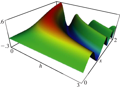
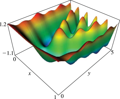
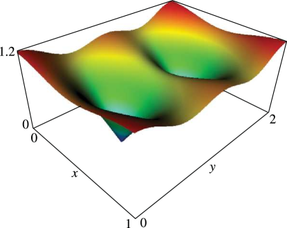
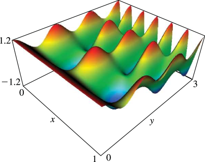
§22.5(ii) Limiting Values of $k$

►If $k\to 0+$, then $K\to \pi /2$ and $K^{\prime }\to \mathrm{\infty }$; if $k\to 1-$, then $K\to \mathrm{\infty }$ and $K^{\prime }\to \pi /2$. … ►Expansions for $K,K^{\prime }$ as $k\to 0$ or $1$ are given in §§19.5, 19.12. … ►

29: 21.4 Graphics

… ►This Riemann matrix originates from the Riemann surface represented by the algebraic curve ${\mu }^3-{\lambda }^7+2{\lambda }^3\mu =0$; compare §21.7(i). ►

…

Figure 21.4.1: $\widehat{\theta }\left(𝐳\right|𝛀)$ parametrized by (21.4.1). The surface plots are of $\widehat{\theta }\left(x+\mathrm{i}y,0\right|𝛀)$, $0\le x\le 1$, $0\le y\le 5$ (suffix 1); $\widehat{\theta }\left(x,y\right|𝛀)$, $0\le x\le 1$, $0\le y\le 1$ (suffix 2); $\widehat{\theta }\left(\mathrm{i}x,\mathrm{i}y\right|𝛀)$, $0\le x\le 5$, $0\le y\le 5$ (suffix 3). …

… ►

►

►

Figure 21.4.2: $\mathrm{\Re }\widehat{\theta }\left(x+\mathrm{i}y,0\right|{𝛀}_1)$, $0\le x\le 1$, $0\le y\le 5$. … Magnify 3D Help

►

►

►

Figure 21.4.3: $\left|\widehat{\theta }\left(x+\mathrm{i}y,0\right|{𝛀}_1)\right|$, $0\le x\le 1$, $0\le y\le 2$. Magnify 3D Help

… ►

►

►

Figure 21.4.5: The real part of a genus 3 scaled Riemann theta function: $\mathrm{\Re }\widehat{\theta }\left(x+\mathrm{i}y,0,0\right|{𝛀}_2)$, $0\le x\le 1$, $0\le y\le 3$. … Magnify 3D Help

30: 10.48 Graphs

… ►

►►

Figure 10.48.1: ${𝗃}_n\left(x\right)$, $n=0(1)4$, $0\le x\le 12$. Magnify

►

►►

Figure 10.48.2: ${𝗒}_n\left(x\right)$, $n=0(1)4$, . Magnify

►

►►

Figure 10.48.3: ${𝗃}_5\left(x\right)$, ${𝗒}_5\left(x\right)$, $\sqrt{{𝗃}_5^2\left(x\right)+{𝗒}_5^2\left(x\right)}$, $0\le x\le 12$. Magnify

►

►►

Figure 10.48.4: ${𝗃}_5^{\prime }\left(x\right)$, ${𝗒}_5^{\prime }\left(x\right)$, $\sqrt{𝗃_5^{\prime }{}_{}{}^2\left(x\right)+𝗒_5^{\prime }{}_{}{}^2\left(x\right)}$, $0\le x\le 12$. Magnify

►

►►

Figure 10.48.5: ${𝗂}_0^{(1)}\left(x\right)$, ${𝗂}_0^{(2)}\left(x\right)$, ${𝗄}_0\left(x\right)$, $0\le x\le 4$. Magnify

…