Jacobi%E2%80%99s

(0.002 seconds)

11—20 of 622 matching pages

11: 19.2 Definitions

… ►Because

s^{2}

is a polynomial, we have … ►

§19.2(ii) Legendre’s Integrals

… ►Legendre’s complementary complete elliptic integrals are defined via … ►

§19.2(iii) Bulirsch’s Integrals

►Bulirsch’s integrals are linear combinations of Legendre’s integrals that are chosen to facilitate computational application of Bartky’s transformation (Bartky (1938)). …

12: 22.21 Tables

§22.21 Tables

►Spenceley and Spenceley (1947) tabulates

\operatorname{sn}\left(Kx,k\right)

\operatorname{cn}\left(Kx,k\right)

\operatorname{dn}\left(Kx,k\right)

\operatorname{am}\left(Kx,k\right)

\mathcal{E}\left(Kx,k\right)

for

\operatorname{arcsin}k=1^{\circ}(1^{\circ})89^{\circ}

and

x=0\left(\tfrac{1}{90}\right)1

to 12D, or 12 decimals of a radian in the case of

\operatorname{am}\left(Kx,k\right)

. … ►Lawden (1989, pp. 280–284 and 293–297) tabulates

\operatorname{sn}\left(x,k\right)

\operatorname{cn}\left(x,k\right)

\operatorname{dn}\left(x,k\right)

\mathcal{E}\left(x,k\right)

\mathrm{Z}\left(x|k\right)

to 5D for

k=0.1(.1)0.9

x=0(.1)X

, where

X

ranges from 1. … ►Zhang and Jin (1996, p. 678) tabulates

\operatorname{sn}\left(Kx,k\right)

\operatorname{cn}\left(Kx,k\right)

\operatorname{dn}\left(Kx,k\right)

for

k=\frac{1}{4},\frac{1}{2}

and

x=0(.1)4

to 7D. …

13: 22.7 Landen Transformations

… ►

22.7.2

\operatorname{sn}\left(z,k\right)=\frac{(1+k_{1})\operatorname{sn}\left(z/(1+k% _{1}),k_{1}\right)}{1+k_{1}{\operatorname{sn}}^{2}\left(z/(1+k_{1}),k_{1}% \right)},

ⓘ

Symbols:: $\operatorname{sn}\left(\NVar{z},\NVar{k}\right)$ : Jacobian elliptic function, $z$ : complex, $k$ : modulus and $k_{1}$ : change of variable
A&S Ref:: 16.12.2
Referenced by:: §22.20(iii)
Permalink:: http://dlmf.nist.gov/22.7.E2
Encodings:: pMML, png, TeX
See also:: Annotations for §22.7(i), §22.7 and Ch.22

►

22.7.3

\operatorname{cn}\left(z,k\right)=\frac{\operatorname{cn}\left(z/(1+k_{1}),k_{% 1}\right)\operatorname{dn}\left(z/(1+k_{1}),k_{1}\right)}{1+k_{1}{% \operatorname{sn}}^{2}\left(z/(1+k_{1}),k_{1}\right)},

ⓘ

Symbols:: $\operatorname{cn}\left(\NVar{z},\NVar{k}\right)$ : Jacobian elliptic function, $\operatorname{dn}\left(\NVar{z},\NVar{k}\right)$ : Jacobian elliptic function, $\operatorname{sn}\left(\NVar{z},\NVar{k}\right)$ : Jacobian elliptic function, $z$ : complex, $k$ : modulus and $k_{1}$ : change of variable
A&S Ref:: 16.12.3
Referenced by:: §22.20(iii)
Permalink:: http://dlmf.nist.gov/22.7.E3
Encodings:: pMML, png, TeX
See also:: Annotations for §22.7(i), §22.7 and Ch.22

►

22.7.4

\operatorname{dn}\left(z,k\right)=\frac{{\operatorname{dn}}^{2}\left(z/(1+k_{1% }),k_{1}\right)-(1-k_{1})}{1+k_{1}-{\operatorname{dn}}^{2}\left(z/(1+k_{1}),k_% {1}\right)}.

ⓘ

Symbols:: $\operatorname{dn}\left(\NVar{z},\NVar{k}\right)$ : Jacobian elliptic function, $z$ : complex, $k$ : modulus and $k_{1}$ : change of variable
A&S Ref:: 16.12.4
Referenced by:: §22.20(iii)
Permalink:: http://dlmf.nist.gov/22.7.E4
Encodings:: pMML, png, TeX
See also:: Annotations for §22.7(i), §22.7 and Ch.22

… ►

22.7.6

\operatorname{sn}\left(z,k\right)=\frac{(1+k_{2}^{\prime})\operatorname{sn}% \left(z/(1+k_{2}^{\prime}),k_{2}\right)\operatorname{cn}\left(z/(1+k_{2}^{% \prime}),k_{2}\right)}{\operatorname{dn}\left(z/(1+k_{2}^{\prime}),k_{2}\right% )},

ⓘ

Symbols:: $\operatorname{cn}\left(\NVar{z},\NVar{k}\right)$ : Jacobian elliptic function, $\operatorname{dn}\left(\NVar{z},\NVar{k}\right)$ : Jacobian elliptic function, $\operatorname{sn}\left(\NVar{z},\NVar{k}\right)$ : Jacobian elliptic function, $z$ : complex, $k$ : modulus, $k_{2}$ : change of variable and $k_{2}^{\prime}$ : change of variable
A&S Ref:: 16.14.2
Permalink:: http://dlmf.nist.gov/22.7.E6
Encodings:: pMML, png, TeX
See also:: Annotations for §22.7(ii), §22.7 and Ch.22

… ►

22.7.8

\operatorname{dn}\left(z,k\right)=\frac{(1-k_{2}^{\prime})({\operatorname{dn}}% ^{2}\left(z/(1+k_{2}^{\prime}),k_{2}\right)+k_{2}^{\prime})}{k_{2}^{2}% \operatorname{dn}\left(z/(1+k_{2}^{\prime}),k_{2}\right)}.

ⓘ

Symbols:: $\operatorname{dn}\left(\NVar{z},\NVar{k}\right)$ : Jacobian elliptic function, $z$ : complex, $k$ : modulus, $k_{2}$ : change of variable and $k_{2}^{\prime}$ : change of variable
A&S Ref:: 16.14.4
Permalink:: http://dlmf.nist.gov/22.7.E8
Encodings:: pMML, png, TeX
See also:: Annotations for §22.7(ii), §22.7 and Ch.22

…

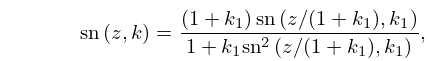
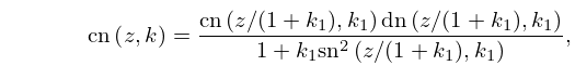
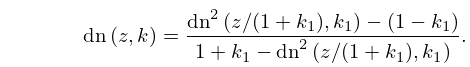
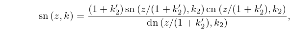
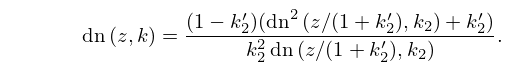
14: 22.4 Periods, Poles, and Zeros

… ►For example, the poles of

\operatorname{sn}\left(z,k\right)

, abbreviated as

\operatorname{sn}

in the following tables, are at

z=2mK+(2n+1)iK^{\prime}

. … ►Then: (a) In any lattice unit cell

\operatorname{pq}\left(z,k\right)

has a simple zero at

z=\mbox{p}

and a simple pole at

z=\mbox{q}

. (b) The difference between p and the nearest q is a half-period of

\operatorname{pq}\left(z,k\right)

. This half-period will be plus or minus a member of the triple

{K,iK^{\prime},K+iK^{\prime}}

; the other two members of this triple are quarter periods of

\operatorname{pq}\left(z,k\right)

. … ►For example,

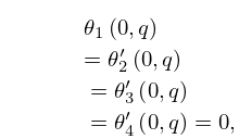
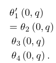
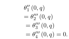
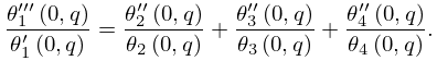
\operatorname{sn}\left(z+K,k\right)=\operatorname{cd}\left(z,k\right)

. …

15: 20.4 Values at $z$ = 0

… ►

20.4.1

\theta_{1}\left(0,q\right)=\theta_{2}'\left(0,q\right)=\theta_{3}'\left(0,q% \right)=\theta_{4}'\left(0,q\right)=0,

ⓘ

Symbols:: $\theta_{\NVar{j}}\left(\NVar{z},\NVar{q}\right)$ : theta function and $q$ : nome
Permalink:: http://dlmf.nist.gov/20.4.E1
Encodings:: pMML, png, TeX
See also:: Annotations for §20.4(i), §20.4 and Ch.20

… ►

Jacobi’s Identity

►

20.4.6

\theta_{1}'\left(0,q\right)=\theta_{2}\left(0,q\right)\theta_{3}\left(0,q% \right)\theta_{4}\left(0,q\right).

ⓘ

Symbols:: $\theta_{\NVar{j}}\left(\NVar{z},\NVar{q}\right)$ : theta function and $q$ : nome
A&S Ref:: 16.28.6
Referenced by:: §20.9(i)
Permalink:: http://dlmf.nist.gov/20.4.E6
Encodings:: pMML, png, TeX
See also:: Annotations for §20.4(i), §20.4(i), §20.4 and Ch.20

… ►

20.4.7

\theta_{1}''\left(0,q\right)=\theta_{2}'''\left(0,q\right)=\theta_{3}'''\left(% 0,q\right)=\theta_{4}'''\left(0,q\right)=0.

ⓘ

Symbols:: $\theta_{\NVar{j}}\left(\NVar{z},\NVar{q}\right)$ : theta function and $q$ : nome
Permalink:: http://dlmf.nist.gov/20.4.E7
Encodings:: pMML, png, TeX
See also:: Annotations for §20.4(ii), §20.4 and Ch.20

… ►

20.4.12

\frac{\theta_{1}'''\left(0,q\right)}{\theta_{1}'\left(0,q\right)}=\frac{\theta% _{2}''\left(0,q\right)}{\theta_{2}\left(0,q\right)}+\frac{\theta_{3}''\left(0,% q\right)}{\theta_{3}\left(0,q\right)}+\frac{\theta_{4}''\left(0,q\right)}{% \theta_{4}\left(0,q\right)}.

ⓘ

Symbols:: $\theta_{\NVar{j}}\left(\NVar{z},\NVar{q}\right)$ : theta function and $q$ : nome
Permalink:: http://dlmf.nist.gov/20.4.E12
Encodings:: pMML, png, TeX
See also:: Annotations for §20.4(ii), §20.4 and Ch.20

16: 20.7 Identities

… ►

20.7.6

{\theta_{4}}^{2}\left(0,q\right)\theta_{1}\left(w+z,q\right)\theta_{1}\left(w-% z,q\right)={\theta_{3}}^{2}\left(w,q\right){\theta_{2}}^{2}\left(z,q\right)-{% \theta_{2}}^{2}\left(w,q\right){\theta_{3}}^{2}\left(z,q\right),

ⓘ

Symbols:: $\theta_{\NVar{j}}\left(\NVar{z},\NVar{q}\right)$ : theta function, $z$ : complex and $q$ : nome
Referenced by:: §20.7(ii)
Permalink:: http://dlmf.nist.gov/20.7.E6
Encodings:: pMML, png, TeX
See also:: Annotations for §20.7(ii), §20.7 and Ch.20

►

20.7.7

{\theta_{4}}^{2}\left(0,q\right)\theta_{2}\left(w+z,q\right)\theta_{2}\left(w-% z,q\right)={\theta_{4}}^{2}\left(w,q\right){\theta_{2}}^{2}\left(z,q\right)-{% \theta_{1}}^{2}\left(w,q\right){\theta_{3}}^{2}\left(z,q\right),

ⓘ

Symbols:: $\theta_{\NVar{j}}\left(\NVar{z},\NVar{q}\right)$ : theta function, $z$ : complex and $q$ : nome
Permalink:: http://dlmf.nist.gov/20.7.E7
Encodings:: pMML, png, TeX
See also:: Annotations for §20.7(ii), §20.7 and Ch.20

►

20.7.8

{\theta_{4}}^{2}\left(0,q\right)\theta_{3}\left(w+z,q\right)\theta_{3}\left(w-% z,q\right)={\theta_{4}}^{2}\left(w,q\right){\theta_{3}}^{2}\left(z,q\right)-{% \theta_{1}}^{2}\left(w,q\right){\theta_{2}}^{2}\left(z,q\right),

ⓘ

Symbols:: $\theta_{\NVar{j}}\left(\NVar{z},\NVar{q}\right)$ : theta function, $z$ : complex and $q$ : nome
Permalink:: http://dlmf.nist.gov/20.7.E8
Encodings:: pMML, png, TeX
See also:: Annotations for §20.7(ii), §20.7 and Ch.20

… ►

20.7.10

\theta_{1}\left(2z,q\right)=2\frac{\theta_{1}\left(z,q\right)\theta_{2}\left(z% ,q\right)\theta_{3}\left(z,q\right)\theta_{4}\left(z,q\right)}{\theta_{2}\left% (0,q\right)\theta_{3}\left(0,q\right)\theta_{4}\left(0,q\right)}.

ⓘ

Symbols:: $\theta_{\NVar{j}}\left(\NVar{z},\NVar{q}\right)$ : theta function, $z$ : complex and $q$ : nome
Permalink:: http://dlmf.nist.gov/20.7.E10
Encodings:: pMML, png, TeX
See also:: Annotations for §20.7(iii), §20.7 and Ch.20

… ►

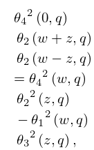
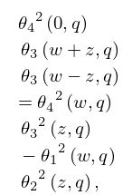
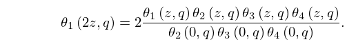
§20.7(v) Watson’s Identities

…

17: 22.1 Special Notation

… ►The functions treated in this chapter are the three principal Jacobian elliptic functions

\operatorname{sn}\left(z,k\right)

\operatorname{cn}\left(z,k\right)

\operatorname{dn}\left(z,k\right)

; the nine subsidiary Jacobian elliptic functions

\operatorname{cd}\left(z,k\right)

\operatorname{sd}\left(z,k\right)

\operatorname{nd}\left(z,k\right)

\operatorname{dc}\left(z,k\right)

\operatorname{nc}\left(z,k\right)

\operatorname{sc}\left(z,k\right)

\operatorname{ns}\left(z,k\right)

\operatorname{ds}\left(z,k\right)

\operatorname{cs}\left(z,k\right)

; the amplitude function

\operatorname{am}\left(x,k\right)

; Jacobi’s epsilon and zeta functions

\mathcal{E}\left(x,k\right)

and

\mathrm{Z}\left(x|k\right)

. … ►The notation

\operatorname{sn}\left(z,k\right)

\operatorname{cn}\left(z,k\right)

\operatorname{dn}\left(z,k\right)

is due to Gudermann (1838), following Jacobi (1827); that for the subsidiary functions is due to Glaisher (1882). Other notations for

\operatorname{sn}\left(z,k\right)

are

\mathrm{sn}(z\mathpunct{|}m)

and

\mathrm{sn}(z,m)

with

m=k^{2}

; see Abramowitz and Stegun (1964) and Walker (1996). …

18: 18.7 Interrelations and Limit Relations

… ►

Ultraspherical and Jacobi

… ►

Chebyshev, Ultraspherical, and Jacobi

… ►

Legendre, Ultraspherical, and Jacobi

… ►

Jacobi $\to$ Laguerre

… ►

Jacobi $\to$ Hermite

…

19: 22.14 Integrals

… ►

22.14.3

\int\operatorname{dn}\left(x,k\right)\,\mathrm{d}x=\operatorname{Arcsin}\left(% \operatorname{sn}\left(x,k\right)\right)=\operatorname{am}\left(x,k\right).

ⓘ

Symbols:: $\operatorname{am}\left(\NVar{x},\NVar{k}\right)$ : Jacobi’s amplitude function, $\operatorname{dn}\left(\NVar{z},\NVar{k}\right)$ : Jacobian elliptic function, $\operatorname{sn}\left(\NVar{z},\NVar{k}\right)$ : Jacobian elliptic function, $\,\mathrm{d}\NVar{x}$ : differential of $x$ , $\int$ : integral, $\operatorname{Arcsin}\NVar{z}$ : general arcsine function, $x$ : real and $k$ : modulus
A&S Ref:: 16.24.3
Permalink:: http://dlmf.nist.gov/22.14.E3
Encodings:: pMML, png, TeX
See also:: Annotations for §22.14(i), §22.14 and Ch.22

… ►See §22.16(i) for

\operatorname{am}\left(z,k\right)

. … ►

22.14.13

\int\frac{\,\mathrm{d}x}{\operatorname{sn}\left(x,k\right)}=\ln\left(\frac{% \operatorname{sn}\left(x,k\right)}{\operatorname{cn}\left(x,k\right)+% \operatorname{dn}\left(x,k\right)}\right),

ⓘ

Symbols:: $\operatorname{cn}\left(\NVar{z},\NVar{k}\right)$ : Jacobian elliptic function, $\operatorname{dn}\left(\NVar{z},\NVar{k}\right)$ : Jacobian elliptic function, $\operatorname{sn}\left(\NVar{z},\NVar{k}\right)$ : Jacobian elliptic function, $\,\mathrm{d}\NVar{x}$ : differential of $x$ , $\int$ : integral, $\ln\NVar{z}$ : principal branch of logarithm function, $x$ : real and $k$ : modulus
Referenced by:: §22.14(iii)
Permalink:: http://dlmf.nist.gov/22.14.E13
Encodings:: pMML, png, TeX
See also:: Annotations for §22.14(iii), §22.14 and Ch.22

►

22.14.14

\int\frac{\operatorname{cn}\left(x,k\right)\,\mathrm{d}x}{\operatorname{sn}% \left(x,k\right)}=\frac{1}{2}\ln\left(\frac{1-\operatorname{dn}\left(x,k\right% )}{1+\operatorname{dn}\left(x,k\right)}\right),

ⓘ

Symbols:: $\operatorname{cn}\left(\NVar{z},\NVar{k}\right)$ : Jacobian elliptic function, $\operatorname{dn}\left(\NVar{z},\NVar{k}\right)$ : Jacobian elliptic function, $\operatorname{sn}\left(\NVar{z},\NVar{k}\right)$ : Jacobian elliptic function, $\,\mathrm{d}\NVar{x}$ : differential of $x$ , $\int$ : integral, $\ln\NVar{z}$ : principal branch of logarithm function, $x$ : real and $k$ : modulus
Permalink:: http://dlmf.nist.gov/22.14.E14
Encodings:: pMML, png, TeX
See also:: Annotations for §22.14(iii), §22.14 and Ch.22

… ►

22.14.18

\int_{0}^{K\left(k\right)}\ln\left(\operatorname{dn}\left(t,k\right)\right)\,% \mathrm{d}t=\tfrac{1}{2}K\left(k\right)\ln k^{\prime}.

ⓘ

Symbols:: $\operatorname{dn}\left(\NVar{z},\NVar{k}\right)$ : Jacobian elliptic function, $K\left(\NVar{k}\right)$ : Legendre’s complete elliptic integral of the first kind, $\,\mathrm{d}\NVar{x}$ : differential of $x$ , $\int$ : integral, $\ln\NVar{z}$ : principal branch of logarithm function, $k$ : modulus and $k^{\prime}$ : complementary modulus
Permalink:: http://dlmf.nist.gov/22.14.E18
Encodings:: pMML, png, TeX
See also:: Annotations for §22.14(iv), §22.14 and Ch.22

…

20: 20.11 Generalizations and Analogs

… ►

§20.11(ii) Ramanujan’s Theta Function and $q$ -Series

… ►This is Jacobi’s inversion problem of §20.9(ii). … ►Each provides an extension of Jacobi’s inversion problem. … ►For

m=1,2,3,4

n=1,2,3,4

, and

m\neq n

, define twelve combined theta functions

\varphi_{m,n}\left(z,q\right)

by …