Jacobi%20nome

SearchAdvancedHelp

(0.001 seconds)

11—20 of 215 matching pages

11: 20.3 Graphics

… ►

§20.3(i) $\theta$-Functions: Real Variable and Real Nome

… ►

►►

Figure 20.3.2: ${\theta }_1(\pi x,q)$, $0\le x\le 2$, $q$ = 0. … Magnify

►

►►

Figure 20.3.3: ${\theta }_2(\pi x,q)$, $0\le x\le 2$, $q$ = 0. … Magnify

… ►

§20.3(ii) $\theta$-Functions: Complex Variable and Real Nome

… ►

►

►

Figure 20.3.18: ${\theta }_1\left(0.1\right|u+\mathrm{i}v)$, $-1\le u\le 1$, $0.005\le v\le 0.5$. …1 of $z$ is chosen arbitrarily since ${\theta }_1$ vanishes identically when $z=0$. Magnify 3D Help

…

12: 20.1 Special Notation

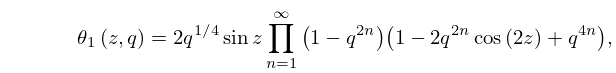
… ►The main functions treated in this chapter are the theta functions ${\theta }_j\left(z\right|\tau )={\theta }_j(z,q)$ where $j=1,2,3,4$ and $q={\mathrm{e}}^{\mathrm{i}\pi \tau }$. When $\tau$ is fixed the notation is often abbreviated in the literature as ${\theta }_j(z)$, or even as simply ${\theta }_j$, it being then understood that the argument is the primary variable. … ►Primes on the $\theta$ symbols indicate derivatives with respect to the argument of the $\theta$ function. … ►Jacobi’s original notation: $\mathrm{\Theta }(z|\tau )$, ${\mathrm{\Theta }}_1(z|\tau )$, $\mathrm{H}(z|\tau )$, ${\mathrm{H}}_1(z|\tau )$, respectively, for ${\theta }_4\left(u\right|\tau )$, ${\theta }_3\left(u\right|\tau )$, ${\theta }_1\left(u\right|\tau )$, ${\theta }_2\left(u\right|\tau )$, where $u=z/{\theta }_3^2\left(0\right|\tau )$. … ►Neville’s notation: ${\theta }_s(z|\tau )$, ${\theta }_c(z|\tau )$, ${\theta }_d(z|\tau )$, ${\theta }_n(z|\tau )$, respectively, for ${\theta }_3^2\left(0\right|\tau ){\theta }_1\left(u\right|\tau )/{\theta }_1^{\prime }\left(0\right|\tau )$, ${\theta }_2\left(u\right|\tau )/{\theta }_2\left(0\right|\tau )$, ${\theta }_3\left(u\right|\tau )/{\theta }_3\left(0\right|\tau )$, ${\theta }_4\left(u\right|\tau )/{\theta }_4\left(0\right|\tau )$, where again $u=z/{\theta }_3^2\left(0\right|\tau )$. …

13: 20.15 Tables

… ►This reference gives ${\theta }_j(x,q)$, $j=1,2,3,4$, and their logarithmic $x$-derivatives to 4D for $x/\pi =0(.1)1$, $\alpha =0(9^{\circ }){90}^{\circ }$, where $\alpha$ is the modular angle given by ►

20.15.1 $$\sin \alpha ={\theta }_2^2(0,q)/{\theta }_3^2(0,q)=k.$$

ⓘ

Defines:

$\alpha$: modular angle (locally)

Symbols:

${\theta }_j(z,q)$: theta function, $\sin z$: sine function and $q$: nome

Referenced by:

§20.15, §20.15

Permalink:

http://dlmf.nist.gov/20.15.E1

Encodings:

pMML, png, TeX

See also:

Annotations for §20.15 and Ch.20

►Spenceley and Spenceley (1947) tabulates ${\theta }_1(x,q)/{\theta }_2(0,q)$, ${\theta }_2(x,q)/{\theta }_2(0,q)$, ${\theta }_3(x,q)/{\theta }_4(0,q)$, ${\theta }_4(x,q)/{\theta }_4(0,q)$ to 12D for $u=0(1^{\circ }){90}^{\circ }$, $\alpha =0(1^{\circ }){89}^{\circ }$, where $u=2x/(\pi {\theta }_3^2(0,q))$ and $\alpha$ is defined by (20.15.1), together with the corresponding values of ${\theta }_2(0,q)$ and ${\theta }_4(0,q)$. ►Lawden (1989, pp. 270–279) tabulates ${\theta }_j(x,q)$, $j=1,2,3,4$, to 5D for $x=0(1^{\circ }){90}^{\circ }$, $q=0.1(.1)0.9$, and also $q$ to 5D for $k^2=0(.01)1$. ►Tables of Neville’s theta functions ${\theta }_s(x,q)$, ${\theta }_c(x,q)$, ${\theta }_d(x,q)$, ${\theta }_n(x,q)$ (see §20.1) and their logarithmic $x$-derivatives are given in Abramowitz and Stegun (1964, pp. 582–585) to 9D for $\epsilon ,\alpha =0(5^{\circ }){90}^{\circ }$, where (in radian measure) $\epsilon =x/{\theta }_3^2(0,q)=\pi x/(2K\left(k\right))$, and $\alpha$ is defined by (20.15.1). …

14: 20.2 Definitions and Periodic Properties

… ►

§20.2(i) Fourier Series

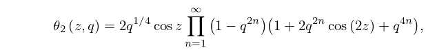
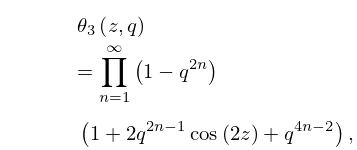
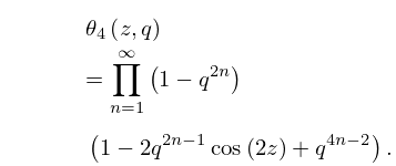
… ►Corresponding expansions for ${\theta }_j^{\prime }\left(z\right|\tau )$, $j=1,2,3,4$, can be found by differentiating (20.2.1)–(20.2.4) with respect to $z$. … ►For fixed $\tau$, each ${\theta }_j\left(z\right|\tau )$ is an entire function of $z$ with period $2\pi$; ${\theta }_1\left(z\right|\tau )$ is odd in $z$ and the others are even. For fixed $z$, each of ${\theta }_1\left(z\right|\tau )/\sin z$, ${\theta }_2\left(z\right|\tau )/\cos z$, ${\theta }_3\left(z\right|\tau )$, and ${\theta }_4\left(z\right|\tau )$ is an analytic function of $\tau$ for $\mathrm{\Im }\tau >0$, with a natural boundary $\mathrm{\Im }\tau =0$, and correspondingly, an analytic function of $q$ for with a natural boundary $\left|q\right|=1$. … ►For $m,n\in \mathbb{Z}$, the $z$-zeros of ${\theta }_j\left(z\right|\tau )$, $j=1,2,3,4$, are $(m+n\tau )\pi$, $(m+\frac{1}{2}+n\tau )\pi$, $(m+\frac{1}{2}+(n+\frac{1}{2})\tau )\pi$, $(m+(n+\frac{1}{2})\tau )\pi$ respectively.

15: 20.5 Infinite Products and Related Results

… ►

20.5.1 $${\theta }_1(z,q)=2q^{1/4}\sin z\prod _{n=1}^{\mathrm{\infty }}\left(1-q^{2n}\right)\left(1-2q^{2n}\cos \left(2z\right)+q^{4n}\right),$$

ⓘ

Symbols:

${\theta }_j(z,q)$: theta function, $\cos z$: cosine function, $\sin z$: sine function, $n$: integer, $z$: complex and $q$: nome

Referenced by:

§20.4(i), §20.5(i), §23.17(iii)

Permalink:

http://dlmf.nist.gov/20.5.E1

Encodings:

pMML, png, TeX

See also:

Annotations for §20.5(i), §20.5 and Ch.20

►

20.5.2 $${\theta }_2(z,q)=2q^{1/4}\cos z\prod _{n=1}^{\mathrm{\infty }}\left(1-q^{2n}\right)\left(1+2q^{2n}\cos \left(2z\right)+q^{4n}\right),$$

ⓘ

Symbols:

${\theta }_j(z,q)$: theta function, $\cos z$: cosine function, $n$: integer, $z$: complex and $q$: nome

Permalink:

http://dlmf.nist.gov/20.5.E2

Encodings:

pMML, png, TeX

See also:

Annotations for §20.5(i), §20.5 and Ch.20

►

20.5.3 $${\theta }_3(z,q)=\prod _{n=1}^{\mathrm{\infty }}\left(1-q^{2n}\right)\left(1+2q^{2n-1}\cos \left(2z\right)+q^{4n-2}\right),$$

ⓘ

Symbols:

${\theta }_j(z,q)$: theta function, $\cos z$: cosine function, $n$: integer, $z$: complex and $q$: nome

Referenced by:

§23.15(ii), §23.17(iii), §23.19

Permalink:

http://dlmf.nist.gov/20.5.E3

Encodings:

pMML, png, TeX

See also:

Annotations for §20.5(i), §20.5 and Ch.20

►

20.5.4 $${\theta }_4(z,q)=\prod _{n=1}^{\mathrm{\infty }}\left(1-q^{2n}\right)\left(1-2q^{2n-1}\cos \left(2z\right)+q^{4n-2}\right).$$

ⓘ

Symbols:

${\theta }_j(z,q)$: theta function, $\cos z$: cosine function, $n$: integer, $z$: complex and $q$: nome

Referenced by:

§20.4(i), §20.5(i)

Permalink:

http://dlmf.nist.gov/20.5.E4

Encodings:

pMML, png, TeX

See also:

Annotations for §20.5(i), §20.5 and Ch.20

… ►

Jacobi’s Triple Product

…

16: 20.9 Relations to Other Functions

… ►

20.9.1 $$k={\theta }_2^2\left(0\right|\tau )/{\theta }_3^2\left(0\right|\tau )$$

ⓘ

Defines:

$k$: modulus (locally)

Symbols:

${\theta }_j\left(z\right|\tau )$: theta function and $\tau$: lattice parameter

Referenced by:

§20.11(iii), §20.9(ii), §23.6(ii)

Permalink:

http://dlmf.nist.gov/20.9.E1

Encodings:

pMML, png, TeX

See also:

Annotations for §20.9(i), §20.9 and Ch.20

… ►

$K\left(k\right)=\frac{1}{2}\pi {\theta }_3^2\left(0\right|\tau ),$

… ►

20.9.3 $$R_F(\frac{{\theta }_2^2(z,q)}{{\theta }_2^2(0,q)},\frac{{\theta }_3^2(z,q)}{{\theta }_3^2(0,q)},\frac{{\theta }_4^2(z,q)}{{\theta }_4^2(0,q)})=\frac{{\theta }_1^{\prime }(0,q)}{{\theta }_1(z,q)}z,$$

ⓘ

Symbols:

$R_F(x,y,z)$: symmetric elliptic integral of first kind, ${\theta }_j(z,q)$: theta function, $z$: complex and $q$: nome

Referenced by:

§19.25(v), §20.9(i)

Permalink:

http://dlmf.nist.gov/20.9.E3

Encodings:

pMML, png, TeX

See also:

Annotations for §20.9(i), §20.9 and Ch.20

►

20.9.4 $$R_F(0,{\theta }_3^4(0,q),{\theta }_4^4(0,q))=\frac{1}{2}\pi ,$$

ⓘ

Symbols:

$R_F(x,y,z)$: symmetric elliptic integral of first kind, ${\theta }_j(z,q)$: theta function, $\pi$: the ratio of the circumference of a circle to its diameter and $q$: nome

Referenced by:

§20.9(i)

Permalink:

http://dlmf.nist.gov/20.9.E4

Encodings:

pMML, png, TeX

See also:

Annotations for §20.9(i), §20.9 and Ch.20

… ►The relations (20.9.1) and (20.9.2) between $k$ and $\tau$ (or $q$) are solutions of Jacobi’s inversion problem; see Baker (1995) and Whittaker and Watson (1927, pp. 480–485). …

17: 22.3 Graphics

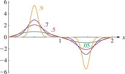
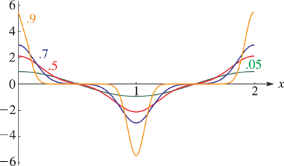
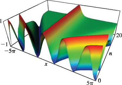
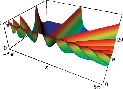
… ►Line graphs of the functions $\mathrm{sn}(x,k)$, $\mathrm{cn}(x,k)$, $\mathrm{dn}(x,k)$, $\mathrm{cd}(x,k)$, $\mathrm{sd}(x,k)$, $\mathrm{nd}(x,k)$, $\mathrm{dc}(x,k)$, $\mathrm{nc}(x,k)$, $\mathrm{sc}(x,k)$, $\mathrm{ns}(x,k)$, $\mathrm{ds}(x,k)$, and $\mathrm{cs}(x,k)$ for representative values of real $x$ and real $k$ illustrating the near trigonometric ($k=0$), and near hyperbolic ($k=1$) limits. 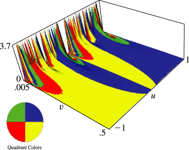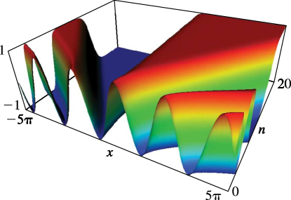… ► $\mathrm{sn}(x,k)$, $\mathrm{cn}(x,k)$, and $\mathrm{dn}(x,k)$ as functions of real arguments $x$ and $k$. … ►

►

►

Figure 22.3.13: $\mathrm{sn}(x,k)$ for $k=1-{\mathrm{e}}^{-n}$, $n=0$ to 20, $-5\pi \le x\le 5\pi$. Magnify 3D Help

►

►

►

Figure 22.3.14: $\mathrm{cn}(x,k)$ for $k=1-{\mathrm{e}}^{-n}$, $n=0$ to 20, $-5\pi \le x\le 5\pi$. Magnify 3D Help

►

►

►

Figure 22.3.15: $\mathrm{dn}(x,k)$ for $k=1-{\mathrm{e}}^{-n}$, $n=0$ to 20, $-5\pi \le x\le 5\pi$. Magnify 3D Help

…

18: 23.15 Definitions

… ►In §§23.15–23.19, $k$ and $k^{\prime }$ $(\in ℂ)$ denote the Jacobi modulus and complementary modulus, respectively, and $q={\mathrm{e}}^{\mathrm{i}\pi \tau }$ ($\mathrm{\Im }\tau >0$) denotes the nome; compare §§20.1 and 22.1. … ►

23.15.6 $$\lambda \left(\tau \right)=\frac{{\theta }_2^4(0,q)}{{\theta }_3^4(0,q)};$$

ⓘ

Defines:

$\lambda \left(\tau \right)$: elliptic modular function

Symbols:

${\theta }_j(z,q)$: theta function, $q$: nome and $\tau$: complex variable

Referenced by:

§20.9(ii), §23.17(iii)

Permalink:

http://dlmf.nist.gov/23.15.E6

Encodings:

pMML, png, TeX

See also:

Annotations for §23.15(ii), §23.15(ii), §23.15 and Ch.23

… ►

23.15.7 $$J\left(\tau \right)=\frac{{\left({\theta }_2^8(0,q)+{\theta }_3^8(0,q)+{\theta }_4^8(0,q)\right)}^3}{54{\left({\theta }_1^{\prime }(0,q)\right)}^8},$$

ⓘ

Defines:

$J\left(\tau \right)$: Klein’s complete invariant

Symbols:

${\theta }_j(z,q)$: theta function, $q$: nome and $\tau$: complex variable

Permalink:

http://dlmf.nist.gov/23.15.E7

Encodings:

pMML, png, TeX

See also:

Annotations for §23.15(ii), §23.15(ii), §23.15 and Ch.23

… ►

23.15.8 $${\theta }_1^{\prime }(0,q)={\partial {\theta }_1(z,q)/\partial z|}_{z=0}.$$

ⓘ

Symbols:

${\theta }_j(z,q)$: theta function, $\frac{\partial f}{\partial x}$: partial derivative of $f$ with respect to $x$ , $\partial x$: partial differential of $x$ , $q$: nome and $z$: complex

Permalink:

http://dlmf.nist.gov/23.15.E8

Encodings:

pMML, png, TeX

See also:

Annotations for §23.15(ii), §23.15(ii), §23.15 and Ch.23

… ►

23.15.9 $$\eta \left(\tau \right)={\left(\frac{1}{2}{\theta }_1^{\prime }(0,q)\right)}^{1/3}={\mathrm{e}}^{\mathrm{i}\pi \tau /12}{\theta }_3\left(\frac{1}{2}\pi (1+\tau )\right|3\tau ).$$

ⓘ

Symbols:

$\eta \left(\tau \right)$: Dedekind’s eta function (or Dedekind modular function), ${\theta }_j(z,q)$: theta function, ${\theta }_j\left(z\right|\tau )$: theta function, $\pi$: the ratio of the circumference of a circle to its diameter, $\mathrm{e}$: base of natural logarithm, $\mathrm{i}$: imaginary unit, $q$: nome and $\tau$: complex variable

Referenced by:

§23.15(ii), §23.15(ii), §23.17(iii)

Permalink:

http://dlmf.nist.gov/23.15.E9

Encodings:

pMML, png, TeX

See also:

Annotations for §23.15(ii), §23.15(ii), §23.15 and Ch.23

…

19: 22.20 Methods of Computation

… ►To compute $\mathrm{sn}$, $\mathrm{cn}$, $\mathrm{dn}$ to 10D when $x=0.8$, $k=0.65$. … ►If either $\tau$ or $q={\mathrm{e}}^{\mathrm{i}\pi \tau }$ is given, then we use $k={\theta }_2^2(0,q)/{\theta }_3^2(0,q)$, $k^{\prime }={\theta }_4^2(0,q)/{\theta }_3^2(0,q)$, $K=\frac{1}{2}\pi {\theta }_3^2(0,q)$, and $K^{\prime }=-\mathrm{i}\tau K$, obtaining the values of the theta functions as in §20.14. … ►

§22.20(vi) Related Functions

… ►Jacobi’s zeta function can then be found by use of (22.16.32). …

20: 22.8 Addition Theorems

… ►

22.8.1 $$\mathrm{sn}(u+v)=\frac{\mathrm{sn}u\mathrm{cn}v\mathrm{dn}v+\mathrm{sn}v\mathrm{cn}u\mathrm{dn}u}{1-k^2{\mathrm{sn}}^{2}u{\mathrm{sn}}^{2}v},$$

ⓘ

Symbols:

$\mathrm{cn}(z,k)$: Jacobian elliptic function, $\mathrm{dn}(z,k)$: Jacobian elliptic function, $\mathrm{sn}(z,k)$: Jacobian elliptic function, $u$: complex, $v$: complex and $k$: modulus

A&S Ref:

16.17.1

Referenced by:

§22.18(iv)

Permalink:

http://dlmf.nist.gov/22.8.E1

Encodings:

pMML, png, TeX

See also:

Annotations for §22.8(i), §22.8 and Ch.22

… ►

22.8.14 $$\mathrm{sn}(u+v)=\frac{\mathrm{sn}u\mathrm{cn}u\mathrm{dn}v+\mathrm{sn}v\mathrm{cn}v\mathrm{dn}u}{\mathrm{cn}u\mathrm{cn}v+\mathrm{sn}u\mathrm{dn}u\mathrm{sn}v\mathrm{dn}v},$$

ⓘ

Symbols:

$\mathrm{cn}(z,k)$: Jacobian elliptic function, $\mathrm{dn}(z,k)$: Jacobian elliptic function, $\mathrm{sn}(z,k)$: Jacobian elliptic function, $u$: complex, $v$: complex and $k$: modulus

Permalink:

http://dlmf.nist.gov/22.8.E14

Encodings:

pMML, png, TeX

See also:

Annotations for §22.8(ii), §22.8 and Ch.22

►

22.8.15 $$\mathrm{cn}(u+v)=\frac{\mathrm{sn}u\mathrm{cn}u\mathrm{dn}v-\mathrm{sn}v\mathrm{cn}v\mathrm{dn}u}{\mathrm{sn}u\mathrm{cn}v\mathrm{dn}v-\mathrm{sn}v\mathrm{cn}u\mathrm{dn}u},$$

ⓘ

Symbols:

$\mathrm{cn}(z,k)$: Jacobian elliptic function, $\mathrm{dn}(z,k)$: Jacobian elliptic function, $\mathrm{sn}(z,k)$: Jacobian elliptic function, $u$: complex, $v$: complex and $k$: modulus

Permalink:

http://dlmf.nist.gov/22.8.E15

Encodings:

pMML, png, TeX

See also:

Annotations for §22.8(ii), §22.8 and Ch.22

… ►

22.8.17 $$\mathrm{dn}(u+v)=\frac{\mathrm{sn}u\mathrm{cn}v\mathrm{dn}u-\mathrm{sn}v\mathrm{cn}u\mathrm{dn}v}{\mathrm{sn}u\mathrm{cn}v\mathrm{dn}v-\mathrm{sn}v\mathrm{cn}u\mathrm{dn}u},$$

ⓘ

Symbols:

$\mathrm{cn}(z,k)$: Jacobian elliptic function, $\mathrm{dn}(z,k)$: Jacobian elliptic function, $\mathrm{sn}(z,k)$: Jacobian elliptic function, $u$: complex, $v$: complex and $k$: modulus

Permalink:

http://dlmf.nist.gov/22.8.E17

Encodings:

pMML, png, TeX

See also:

Annotations for §22.8(ii), §22.8 and Ch.22

… ►

22.8.23

ⓘ

Symbols:

$\mathrm{cn}(z,k)$: Jacobian elliptic function, $\mathrm{dn}(z,k)$: Jacobian elliptic function, $\mathrm{sn}(z,k)$: Jacobian elliptic function, $det$: determinant, $z$: complex and $k$: modulus

Permalink:

http://dlmf.nist.gov/22.8.E23

Encodings:

pMML, png, TeX

See also:

Annotations for §22.8(iii), §22.8 and Ch.22

…