Jacobi imaginary transformation

(0.004 seconds)

1—10 of 24 matching pages

$\operatorname{sn}\left(iz,k\right)$ $\;=\;$	$i\operatorname{sc}\left(z,k^{\prime}\right)$	$\operatorname{dc}\left(iz,k\right)$ $\;=\;$	$\operatorname{dn}\left(z,k^{\prime}\right)$
…

2: 29.10 Lamé Functions with Imaginary Periods

§29.10 Lamé Functions with Imaginary Periods

… ►

29.10.2

z^{\prime}=\mathrm{i}(z-K-\mathrm{i}{K^{\prime}}),

ⓘ

Symbols:: ${K^{\prime}}\left(\NVar{k}\right)$ : Legendre’s complementary complete elliptic integral of the first kind, $K\left(\NVar{k}\right)$ : Legendre’s complete elliptic integral of the first kind, $\mathrm{i}$ : imaginary unit, $z$ : complex variable and $k$ : real parameter
Permalink:: http://dlmf.nist.gov/29.10.E2
Encodings:: pMML, png, TeX
See also:: Annotations for §29.10 and Ch.29

►transform (29.2.1) into … ►

\mathit{Ec}^{2m}_{\nu}\left(\mathrm{i}(z-K-\mathrm{i}{K^{\prime}}),{k^{\prime}% }^{2}\right),

… ►The first and the fourth functions have period

2\mathrm{i}{K^{\prime}}

; the second and the third have period

4\mathrm{i}{K^{\prime}}

. …

3: 14.31 Other Applications

… ►

§14.31(ii) Conical Functions

►The conical functions

\mathsf{P}^{m}_{-\frac{1}{2}+i\tau}\left(x\right)

appear in boundary-value problems for the Laplace equation in toroidal coordinates (§14.19(i)) for regions bounded by cones, by two intersecting spheres, or by one or two confocal hyperboloids of revolution (Kölbig (1981)). These functions are also used in the Mehler–Fock integral transform (§14.20(vi)) for problems in potential and heat theory, and in elementary particle physics (Sneddon (1972, Chapter 7) and Braaksma and Meulenbeld (1967)). The conical functions and Mehler–Fock transform generalize to Jacobi functions and the Jacobi transform; see Koornwinder (1984a) and references therein. …

4: 20.14 Methods of Computation

… ►For instance, the first three terms of (20.2.1) give the value of

\theta_{1}\left(2-i\middle|i\right)

(

=\theta_{1}\left(2-i,e^{-\pi}\right)

) to 12 decimal places. ►For values of

\left|q\right|

near

1

the transformations of §20.7(viii) can be used to replace

\tau

with a value that has a larger imaginary part and hence a smaller value of

\left|q\right|

. For instance, to find

\theta_{3}\left(z,0.9\right)

we use (20.7.32) with

q=0.9=e^{i\pi\tau}

\tau=-i\ln\left(0.9\right)/\pi

. …Hence the first term of the series (20.2.3) for

\theta_{3}\left(z\tau^{\prime}\middle|\tau^{\prime}\right)

suffices for most purposes. In theory, starting from any value of

\tau

, a finite number of applications of the transformations

\tau\to\tau+1

and

\tau\to-1/\tau

will result in a value of

\tau

with

\Im\tau\geq\sqrt{3}/2

; see §23.18. …

5: 20.10 Integrals

… ►

20.10.1

\int_{0}^{\infty}x^{s-1}\theta_{2}\left(0\middle|ix^{2}\right)\,\mathrm{d}x=2^% {s}(1-2^{-s})\pi^{-s/2}\Gamma\left(\tfrac{1}{2}s\right)\zeta\left(s\right),

\Re s>1

ⓘ

Symbols:: $\Gamma\left(\NVar{z}\right)$ : gamma function, $\theta_{\NVar{j}}\left(\NVar{z}\middle|\NVar{\tau}\right)$ : theta function, $\zeta\left(\NVar{s}\right)$ : Riemann zeta function, $\pi$ : the ratio of the circumference of a circle to its diameter, $\,\mathrm{d}\NVar{x}$ : differential of $x$ , $\mathrm{i}$ : imaginary unit, $\int$ : integral and $\Re$ : real part
Keywords:: Mellin transform
Referenced by:: §20.10(i), Erratum (V1.1.5) for §20.10(i)
Permalink:: http://dlmf.nist.gov/20.10.E1
Encodings:: pMML, png, TeX
Modification (effective with 1.1.5):: Originally the constraint was $\Re s>2$ . This can be relaxed to $\Re s>1$ because $\theta_{2}\left(0\middle|ix^{2}\right)=x^{-1}\theta_{4}\left(0\middle|ix^{-2}% \right)\sim x^{-1}$ as $x\to 0+$ , which follows from (20.7.31) and (20.4.5).
See also:: Annotations for §20.10(i), §20.10 and Ch.20

►

20.10.2

\int_{0}^{\infty}x^{s-1}(\theta_{3}\left(0\middle|ix^{2}\right)-1)\,\mathrm{d}% x=\pi^{-s/2}\Gamma\left(\tfrac{1}{2}s\right)\zeta\left(s\right),

\Re s>1

ⓘ

Symbols:: $\Gamma\left(\NVar{z}\right)$ : gamma function, $\theta_{\NVar{j}}\left(\NVar{z}\middle|\NVar{\tau}\right)$ : theta function, $\zeta\left(\NVar{s}\right)$ : Riemann zeta function, $\pi$ : the ratio of the circumference of a circle to its diameter, $\,\mathrm{d}\NVar{x}$ : differential of $x$ , $\mathrm{i}$ : imaginary unit, $\int$ : integral and $\Re$ : real part
Keywords:: Mellin transform
Referenced by:: §20.10(i), Erratum (V1.1.5) for §20.10(i)
Permalink:: http://dlmf.nist.gov/20.10.E2
Encodings:: pMML, png, TeX
Modification (effective with 1.1.5):: Originally the constraint was $\Re s>2$ . This can be relaxed to $\Re s>1$ because $\theta_{3}\left(0\middle|ix^{2}\right)=x^{-1}\theta_{3}\left(0\middle|ix^{-2}% \right)\sim x^{-1}$ as $x\to 0+$ , which follows from (20.7.32) and (20.4.4).
See also:: Annotations for §20.10(i), §20.10 and Ch.20

►

20.10.3

\int_{0}^{\infty}x^{s-1}(1-\theta_{4}\left(0\middle|ix^{2}\right))\,\mathrm{d}% x=(1-2^{1-s})\pi^{-s/2}\Gamma\left(\tfrac{1}{2}s\right)\zeta\left(s\right),

\Re s>0

ⓘ

Symbols:: $\Gamma\left(\NVar{z}\right)$ : gamma function, $\theta_{\NVar{j}}\left(\NVar{z}\middle|\NVar{\tau}\right)$ : theta function, $\zeta\left(\NVar{s}\right)$ : Riemann zeta function, $\pi$ : the ratio of the circumference of a circle to its diameter, $\,\mathrm{d}\NVar{x}$ : differential of $x$ , $\mathrm{i}$ : imaginary unit, $\int$ : integral and $\Re$ : real part
Keywords:: Mellin transform
Referenced by:: §20.10(i), Erratum (V1.1.5) for §20.10(i)
Permalink:: http://dlmf.nist.gov/20.10.E3
Encodings:: pMML, png, TeX
Modification (effective with 1.1.5):: Originally the constraint was $\Re s>2$ . This can be relaxed to $\Re s>0$ because $1-\theta_{4}\left(0\middle|ix^{2}\right)=1-x^{-1}\theta_{2}\left(0\middle|ix^{% -2}\right)\sim 1$ as $x\to 0+$ , which follows from (20.7.33) and (20.4.3).
See also:: Annotations for §20.10(i), §20.10 and Ch.20

…

6: 20.7 Identities

… ►

20.7.33

(-i\tau)^{1/2}\theta_{4}\left(z\middle|\tau\right)=\exp\left(i\tau^{\prime}z^{% 2}/\pi\right)\theta_{2}\left(z\tau^{\prime}\middle|\tau^{\prime}\right).

ⓘ

Symbols:: $\theta_{\NVar{j}}\left(\NVar{z}\middle|\NVar{\tau}\right)$ : theta function, $\pi$ : the ratio of the circumference of a circle to its diameter, $\exp\NVar{z}$ : exponential function, $\mathrm{i}$ : imaginary unit, $z$ : complex and $\tau$ : lattice parameter
Referenced by:: (20.10.3), §20.13
Permalink:: http://dlmf.nist.gov/20.7.E33
Encodings:: pMML, png, TeX
See also:: Annotations for §20.7(viii), §20.7 and Ch.20

…

7: 15.9 Relations to Other Functions

… ►

Jacobi

… ►

§15.9(ii) Jacobi Function

… ►The Jacobi transform is defined as …with inverse … …

8: 29.18 Mathematical Applications

… ►when transformed to sphero-conal coordinates

r,\beta,\gamma

: ►

x=kr\operatorname{sn}\left(\beta,k\right)\operatorname{sn}\left(\gamma,k\right),

►

y=\mathrm{i}\frac{k}{k^{\prime}}r\operatorname{cn}\left(\beta,k\right)% \operatorname{cn}\left(\gamma,k\right),

… ►The wave equation (29.18.1), when transformed to ellipsoidal coordinates

\alpha,\beta,\gamma

: … ►

z=\frac{\mathrm{i}}{kk^{\prime}}\operatorname{dn}\left(\alpha,k\right)% \operatorname{dn}\left(\beta,k\right)\operatorname{dn}\left(\gamma,k\right),

…

9: 15.17 Mathematical Applications

… ►The logarithmic derivatives of some hypergeometric functions for which quadratic transformations exist (§15.8(iii)) are solutions of Painlevé equations. … ►

§15.17(iii) Group Representations

►For harmonic analysis it is more natural to represent hypergeometric functions as a Jacobi function (§15.9(ii)). …Harmonic analysis can be developed for the Jacobi transform either as a generalization of the Fourier-cosine transform (§1.14(ii)) or as a specialization of a group Fourier transform. … ►Quadratic transformations give insight into the relation of elliptic integrals to the arithmetic-geometric mean (§19.22(ii)). …

10: 23.15 Definitions

… ►In §§23.15–23.19,

k

and

k^{\prime}

(\in\mathbb{C})

denote the Jacobi modulus and complementary modulus, respectively, and

q=e^{i\pi\tau}

(

\Im\tau>0

) denotes the nome; compare §§20.1 and 22.1. … ►Also

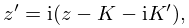
\mathcal{A}

denotes a bilinear transformation on

\tau

, given by …The set of all bilinear transformations of this form is denoted by SL

(2,\mathbb{Z})

(Serre (1973, p. 77)). … ►In (23.15.9) the branch of the cube root is chosen to agree with the second equality; in particular, when

\tau

lies on the positive imaginary axis the cube root is real and positive. …