Gauss%E2%80%93Legendre formula

SearchAdvancedHelp

(0.002 seconds)

21—30 of 410 matching pages

21: 35.7 Gaussian Hypergeometric Function of Matrix Argument

… ►

Gauss Formula

… ►

Reflection Formula

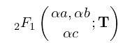
… ►Subject to the conditions (a)–(c), the function $f(𝐓)={}_2{}^{}F_1^{}(a,b;c;𝐓)$ is the unique solution of each partial differential equation … ►Systems of partial differential equations for the ${}_0{}^{}F_1^{}$ (defined in §35.8) and ${}_1{}^{}F_1^{}$ functions of matrix argument can be obtained by applying (35.8.9) and (35.8.10) to (35.7.9). … ►

35.7.10 $${}_2{}^{}F_1^{}(\genfrac{}{}{0pt}{}{\alpha a,\alpha b}{\alpha c};𝐓)$$

ⓘ

Symbols:

${}_p{}^{}F_q^{}(a_1,\mathrm{\dots },a_p;b_1,\mathrm{\dots },b_q;𝐓)$ or ${}_p{}^{}F_q^{}(\genfrac{}{}{0pt}{}{a_1,\mathrm{\dots },a_p}{b_1,\mathrm{\dots },b_q};𝐓)$: generalized hypergeometric function of matrix argument, $a$: complex variable, $𝐓$: real symmetric $m\times m$ matrix, $b$: complex variable, $c$: complex variable and $\alpha \to \mathrm{\infty }$: parameter

Permalink:

http://dlmf.nist.gov/35.7.E10

Encodings:

pMML, png, TeX

See also:

Annotations for §35.7(iv), §35.7 and Ch.35

…

22: 19.5 Maclaurin and Related Expansions

§19.5 Maclaurin and Related Expansions

… ►

19.5.1 $$K\left(k\right)=\frac{\pi }{2}\sum _{m=0}^{\mathrm{\infty }}\frac{{\left(\frac{1}{2}\right)}_m{\left(\frac{1}{2}\right)}_m}{m!m!}{k}^{2m}=\frac{\pi }{2}{}_2{}^{}F_1^{}(\genfrac{}{}{0pt}{}{\frac{1}{2},\frac{1}{2}}{1};k^2),$$

ⓘ

Symbols:

${}_2{}^{}F_1^{}(a,b;c;z)$: $=F(a,b;c;z)$ notation for Gauss’ hypergeometric function, ${\left(a\right)}_n$: Pochhammer’s symbol (or shifted factorial), $\pi$: the ratio of the circumference of a circle to its diameter, $K\left(k\right)$: Legendre’s complete elliptic integral of the first kind, $!$: factorial (as in $n!$), $m$: nonnegative integer and $k$: real or complex modulus

Source:

Carlson (1961b, (2.4))

Referenced by:

§19.36(iv), §19.5

Permalink:

http://dlmf.nist.gov/19.5.E1

Encodings:

pMML, png, TeX

See also:

Annotations for §19.5 and Ch.19

►where ${}_2{}^{}F_1^{}$ is the Gauss hypergeometric function (§§15.1 and 15.2(i)). … … ►

23: 16.16 Transformations of Variables

… ►

§16.16(i) Reduction Formulas

►

16.16.1 $$F_1(\alpha ;\beta ,{\beta }^{\prime };\beta +{\beta }^{\prime };x,y)={(1-y)}^{-\alpha }{}_2{}^{}F_1^{}(\genfrac{}{}{0pt}{}{\alpha ,\beta }{\beta +{\beta }^{\prime }};\frac{x-y}{1-y}),$$

ⓘ

Symbols:

$F_1(\alpha ;\beta ,{\beta }^{\prime };\gamma ;x,y)$: first Appell function and ${}_2{}^{}F_1^{}(a,b;c;z)$: $=F(a,b;c;z)$ notation for Gauss’ hypergeometric function

Permalink:

http://dlmf.nist.gov/16.16.E1

Encodings:

pMML, png, TeX

See also:

Annotations for §16.16(i), §16.16 and Ch.16

►

16.16.2 $$F_2(\alpha ;\beta ,{\beta }^{\prime };\gamma ,{\beta }^{\prime };x,y)={(1-y)}^{-\alpha }{}_2{}^{}F_1^{}(\genfrac{}{}{0pt}{}{\alpha ,\beta }{\gamma };\frac{x}{1-y}),$$

ⓘ

Symbols:

$F_2(\alpha ;\beta ,{\beta }^{\prime };\gamma ,{\gamma }^{\prime };x,y)$: second Appell function and ${}_2{}^{}F_1^{}(a,b;c;z)$: $=F(a,b;c;z)$ notation for Gauss’ hypergeometric function

Permalink:

http://dlmf.nist.gov/16.16.E2

Encodings:

pMML, png, TeX

See also:

Annotations for §16.16(i), §16.16 and Ch.16

… ►

16.16.5 $$F_3(\alpha ,\gamma -\alpha ;\beta ,\gamma -\beta ;\gamma ;x,y)={(1-y)}^{\alpha +\beta -\gamma }{}_2{}^{}F_1^{}(\genfrac{}{}{0pt}{}{\alpha ,\beta }{\gamma };x+y-xy),$$

ⓘ

Symbols:

$F_3(\alpha ,{\alpha }^{\prime };\beta ,{\beta }^{\prime };\gamma ;x,y)$: third Appell function and ${}_2{}^{}F_1^{}(a,b;c;z)$: $=F(a,b;c;z)$ notation for Gauss’ hypergeometric function

Permalink:

http://dlmf.nist.gov/16.16.E5

Encodings:

pMML, png, TeX

See also:

Annotations for §16.16(i), §16.16 and Ch.16

… ►See Erdélyi et al. (1953a, §5.10) for these and further reduction formulas. …

24: 19.2 Definitions

… ►

§19.2(ii) Legendre’s Integrals

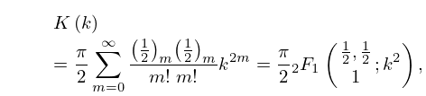
… ►Legendre’s complementary complete elliptic integrals are defined via … ►Bulirsch’s integrals are linear combinations of Legendre’s integrals that are chosen to facilitate computational application of Bartky’s transformation (Bartky (1938)). … ►Lastly, corresponding to Legendre’s incomplete integral of the third kind we have … ►Formulas involving $\mathrm{\Pi }(\varphi ,{\alpha }^2,k)$ that are customarily different for circular cases, ordinary hyperbolic cases, and (hyperbolic) Cauchy principal values, are united in a single formula by using $R_C(x,y)$. …

25: 18.26 Wilson Class: Continued

… ►

18.26.2 $$S_n(y^2;a,b,c)={\left(a+b\right)}_n{\left(a+c\right)}_n{}_3{}^{}F_2^{}(\genfrac{}{}{0pt}{}{-n,a+iy,a-iy}{a+b,a+c};1).$$

ⓘ

Symbols:

${}_p{}^{}F_q^{}(a_1,\mathrm{\dots },a_p;b_1,\mathrm{\dots },b_q;z)$ or ${}_p{}^{}F_q^{}(\genfrac{}{}{0pt}{}{a_1,\mathrm{\dots },a_p}{b_1,\mathrm{\dots },b_q};z)$: alternatively ${}_p{}^{}F_q^{}(𝐚;𝐛;z)$ or ${}_p{}^{}F_q^{}(\genfrac{}{}{0pt}{}{𝐚}{𝐛};z)$
generalized hypergeometric function, ${\left(a\right)}_n$: Pochhammer’s symbol (or shifted factorial), $S_n(x;a,b,c)$: continuous dual Hahn polynomial, $y$: real variable and $n$: nonnegative integer

Referenced by:

§18.26(i), §18.26(ii), §18.26(iv)

Permalink:

http://dlmf.nist.gov/18.26.E2

Encodings:

pMML, png, TeX

See also:

Annotations for §18.26(i), §18.26 and Ch.18

… ►See Koekoek et al. (2010, Chapter 9) for further formulas. … ►For the hypergeometric function ${}_2{}^{}F_1^{}$ see §§15.1 and 15.2(i). … ►

18.26.18 $${}_2{}^{}F_1^{}(\genfrac{}{}{0pt}{}{a+\mathrm{i}y,d+\mathrm{i}y}{a+d};z){}_2{}^{}F_1^{}(\genfrac{}{}{0pt}{}{b-\mathrm{i}y,c-\mathrm{i}y}{b+c};z)=\sum _{n=0}^{\mathrm{\infty }}\frac{W_n(y^2;a,b,c,d)}{{\left(a+d\right)}_n{\left(b+c\right)}_{n}n!}{z}^n,$$ .

ⓘ

Symbols:

${}_2{}^{}F_1^{}(a,b;c;z)$: $=F(a,b;c;z)$ notation for Gauss’ hypergeometric function, ${\left(a\right)}_n$: Pochhammer’s symbol (or shifted factorial), $W_n(x;a,b,c,d)$: Wilson polynomial, $!$: factorial (as in $n!$), $\mathrm{i}$: imaginary unit, $y$: real variable, $z$: complex variable and $n$: nonnegative integer

Referenced by:

§18.23, §18.26(iv)

Permalink:

http://dlmf.nist.gov/18.26.E18

Encodings:

pMML, png, TeX

See also:

Annotations for §18.26(iv), §18.26(iv), §18.26 and Ch.18

… ►

18.26.19 $${(1-z)}^{-c+\mathrm{i}y}{}_2{}^{}F_1^{}(\genfrac{}{}{0pt}{}{a+\mathrm{i}y,b+\mathrm{i}y}{a+b};z)=\sum _{n=0}^{\mathrm{\infty }}\frac{S_n(y^2;a,b,c)}{{\left(a+b\right)}_{n}n!}{z}^n,$$ .

ⓘ

Symbols:

${}_2{}^{}F_1^{}(a,b;c;z)$: $=F(a,b;c;z)$ notation for Gauss’ hypergeometric function, ${\left(a\right)}_n$: Pochhammer’s symbol (or shifted factorial), $S_n(x;a,b,c)$: continuous dual Hahn polynomial, $!$: factorial (as in $n!$), $\mathrm{i}$: imaginary unit, $y$: real variable, $z$: complex variable and $n$: nonnegative integer

Referenced by:

§18.26(iv)

Permalink:

http://dlmf.nist.gov/18.26.E19

Encodings:

pMML, png, TeX

See also:

Annotations for §18.26(iv), §18.26(iv), §18.26 and Ch.18

…

26: 15.10 Hypergeometric Differential Equation

… ►

$f_1(z)=F({\displaystyle \genfrac{}{}{0pt}{}{a,b}{c}};z),$

… ►

$f_1(z)=F({\displaystyle \genfrac{}{}{0pt}{}{a,b}{a+b+1-c}};1-z),$

… ►(b) If $c$ equals $n=1,2,3,\mathrm{\dots }$, and $a\ne 1,2,\mathrm{\dots },n-1$, then fundamental solutions in the neighborhood of $z=0$ are given by $F(a,b;n;z)$ and … ►

§15.10(ii) Kummer’s 24 Solutions and Connection Formulas

… ►The $\left(\genfrac{}{}{0.0pt}{}{6}{3}\right)=20$ connection formulas for the principal branches of Kummer’s solutions are: …

27: 27.2 Functions

… ►Gauss and Legendre conjectured that $\pi \left(x\right)$ is asymptotic to $x/\ln x$ as $x\to \mathrm{\infty }$: …(See Gauss (1863, Band II, pp. 437–477) and Legendre (1808, p. 394).) … ►

Table 27.2.1: Primes.

► ►►

$n$	$p_n$	$p_{n+10}$	$p_{n+20}$	$p_{n+30}$	$p_{n+40}$	$p_{n+50}$	$p_{n+60}$	$p_{n+70}$	$p_{n+80}$	$p_{n+90}$
…

►

►

Table 27.2.2: Functions related to division.

► ►►►

$n$	$\varphi \left(n\right)$	$d\left(n\right)$	$\sigma \left(n\right)$	$n$	$\varphi \left(n\right)$	$d\left(n\right)$	$\sigma \left(n\right)$	$n$	$\varphi \left(n\right)$	$d\left(n\right)$	$\sigma \left(n\right)$	$n$	$\varphi \left(n\right)$	$d\left(n\right)$	$\sigma \left(n\right)$
…
11	10	2	12	24	8	8	60	37	36	2	38	50	20	6	93
…

►

28: 19.15 Advantages of Symmetry

… ►Symmetry in $x,y,z$ of $R_F(x,y,z)$, $R_G(x,y,z)$, and $R_J(x,y,z,p)$ replaces the five transformations (19.7.2), (19.7.4)–(19.7.7) of Legendre’s integrals; compare (19.25.17). Symmetry unifies the Landen transformations of §19.8(ii) with the Gauss transformations of §19.8(iii), as indicated following (19.22.22) and (19.36.9). (19.21.12) unifies the three transformations in §19.7(iii) that change the parameter of Legendre’s third integral. … ►These reduction theorems, unknown in the Legendre theory, allow symbolic integration without imposing conditions on the parameters and the limits of integration (see §19.29(ii)). …

29: 15.3 Graphics

… ►

►►

Figure 15.3.1: $F(\frac{4}{3},\frac{9}{16};\frac{14}{5};x),-100\le x\le 1$. Magnify

►

►►

Figure 15.3.2: $F(5,-10;1;x),-0.023\le x\le 1$. Magnify

►

►►

Figure 15.3.3: $F(1,-10;10;x),-3\le x\le 1$. Magnify

►

►►

Figure 15.3.4: $F(5,10;1;x),-1\le x\le 0.022$. Magnify

… ►

►

►

Figure 15.3.5: $F(\frac{4}{3},\frac{9}{16};\frac{14}{5};x+\mathrm{i}y),0\le x\le 2,-0.5\le y\le 0.5$. … Magnify 3D Help

…

30: 35.9 Applications

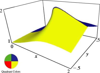
… ►In multivariate statistical analysis based on the multivariate normal distribution, the probability density functions of many random matrices are expressible in terms of generalized hypergeometric functions of matrix argument ${}_p{}^{}F_q^{}$, with $p\le 2$ and $q\le 1$. … ►For other statistical applications of ${}_p{}^{}F_q^{}$ functions of matrix argument see Perlman and Olkin (1980), Groeneboom and Truax (2000), Bhaumik and Sarkar (2002), Richards (2004) (monotonicity of power functions of multivariate statistical test criteria), Bingham et al. (1992) (Procrustes analysis), and Phillips (1986) (exact distributions of statistical test criteria). These references all use results related to the integral formulas (35.4.7) and (35.5.8). …