Gauss%E2%80%93Laguerre%20formula

SearchAdvancedHelp

(0.002 seconds)

21—30 of 391 matching pages

21: 16.16 Transformations of Variables

… ►

§16.16(i) Reduction Formulas

►

16.16.1 $$F_1(\alpha ;\beta ,{\beta }^{\prime };\beta +{\beta }^{\prime };x,y)={(1-y)}^{-\alpha }{}_2{}^{}F_1^{}(\genfrac{}{}{0pt}{}{\alpha ,\beta }{\beta +{\beta }^{\prime }};\frac{x-y}{1-y}),$$

ⓘ

Symbols:

$F_1(\alpha ;\beta ,{\beta }^{\prime };\gamma ;x,y)$: first Appell function and ${}_2{}^{}F_1^{}(a,b;c;z)$: $=F(a,b;c;z)$ notation for Gauss’ hypergeometric function

Permalink:

http://dlmf.nist.gov/16.16.E1

Encodings:

pMML, png, TeX

See also:

Annotations for §16.16(i), §16.16 and Ch.16

►

16.16.2 $$F_2(\alpha ;\beta ,{\beta }^{\prime };\gamma ,{\beta }^{\prime };x,y)={(1-y)}^{-\alpha }{}_2{}^{}F_1^{}(\genfrac{}{}{0pt}{}{\alpha ,\beta }{\gamma };\frac{x}{1-y}),$$

ⓘ

Symbols:

$F_2(\alpha ;\beta ,{\beta }^{\prime };\gamma ,{\gamma }^{\prime };x,y)$: second Appell function and ${}_2{}^{}F_1^{}(a,b;c;z)$: $=F(a,b;c;z)$ notation for Gauss’ hypergeometric function

Permalink:

http://dlmf.nist.gov/16.16.E2

Encodings:

pMML, png, TeX

See also:

Annotations for §16.16(i), §16.16 and Ch.16

… ►

16.16.5 $$F_3(\alpha ,\gamma -\alpha ;\beta ,\gamma -\beta ;\gamma ;x,y)={(1-y)}^{\alpha +\beta -\gamma }{}_2{}^{}F_1^{}(\genfrac{}{}{0pt}{}{\alpha ,\beta }{\gamma };x+y-xy),$$

ⓘ

Symbols:

$F_3(\alpha ,{\alpha }^{\prime };\beta ,{\beta }^{\prime };\gamma ;x,y)$: third Appell function and ${}_2{}^{}F_1^{}(a,b;c;z)$: $=F(a,b;c;z)$ notation for Gauss’ hypergeometric function

Permalink:

http://dlmf.nist.gov/16.16.E5

Encodings:

pMML, png, TeX

See also:

Annotations for §16.16(i), §16.16 and Ch.16

… ►See Erdélyi et al. (1953a, §5.10) for these and further reduction formulas. …

22: 27.2 Functions

… ►Euclid’s Elements (Euclid (1908, Book IX, Proposition 20)) gives an elegant proof that there are infinitely many primes. … ►Gauss and Legendre conjectured that $\pi \left(x\right)$ is asymptotic to $x/\ln x$ as $x\to \mathrm{\infty }$: …(See Gauss (1863, Band II, pp. 437–477) and Legendre (1808, p. 394).) … ►

Table 27.2.1: Primes.

► ►►

$n$	$p_n$	$p_{n+10}$	$p_{n+20}$	$p_{n+30}$	$p_{n+40}$	$p_{n+50}$	$p_{n+60}$	$p_{n+70}$	$p_{n+80}$	$p_{n+90}$
…

►

►

Table 27.2.2: Functions related to division.

► ►►►

$n$	$\varphi \left(n\right)$	$d\left(n\right)$	$\sigma \left(n\right)$	$n$	$\varphi \left(n\right)$	$d\left(n\right)$	$\sigma \left(n\right)$	$n$	$\varphi \left(n\right)$	$d\left(n\right)$	$\sigma \left(n\right)$	$n$	$\varphi \left(n\right)$	$d\left(n\right)$	$\sigma \left(n\right)$
…
11	10	2	12	24	8	8	60	37	36	2	38	50	20	6	93
…

►

23: 18.26 Wilson Class: Continued

… ►

18.26.2 $$S_n(y^2;a,b,c)={\left(a+b\right)}_n{\left(a+c\right)}_n{}_3{}^{}F_2^{}(\genfrac{}{}{0pt}{}{-n,a+iy,a-iy}{a+b,a+c};1).$$

ⓘ

Symbols:

${}_p{}^{}F_q^{}(a_1,\mathrm{\dots },a_p;b_1,\mathrm{\dots },b_q;z)$ or ${}_p{}^{}F_q^{}(\genfrac{}{}{0pt}{}{a_1,\mathrm{\dots },a_p}{b_1,\mathrm{\dots },b_q};z)$: alternatively ${}_p{}^{}F_q^{}(𝐚;𝐛;z)$ or ${}_p{}^{}F_q^{}(\genfrac{}{}{0pt}{}{𝐚}{𝐛};z)$
generalized hypergeometric function, ${\left(a\right)}_n$: Pochhammer’s symbol (or shifted factorial), $S_n(x;a,b,c)$: continuous dual Hahn polynomial, $y$: real variable and $n$: nonnegative integer

Referenced by:

§18.26(i), §18.26(ii), §18.26(iv)

Permalink:

http://dlmf.nist.gov/18.26.E2

Encodings:

pMML, png, TeX

See also:

Annotations for §18.26(i), §18.26 and Ch.18

… ►See Koekoek et al. (2010, Chapter 9) for further formulas. … ►For the hypergeometric function ${}_2{}^{}F_1^{}$ see §§15.1 and 15.2(i). … ►

18.26.18 $${}_2{}^{}F_1^{}(\genfrac{}{}{0pt}{}{a+\mathrm{i}y,d+\mathrm{i}y}{a+d};z){}_2{}^{}F_1^{}(\genfrac{}{}{0pt}{}{b-\mathrm{i}y,c-\mathrm{i}y}{b+c};z)=\sum _{n=0}^{\mathrm{\infty }}\frac{W_n(y^2;a,b,c,d)}{{\left(a+d\right)}_n{\left(b+c\right)}_{n}n!}{z}^n,$$ .

ⓘ

Symbols:

${}_2{}^{}F_1^{}(a,b;c;z)$: $=F(a,b;c;z)$ notation for Gauss’ hypergeometric function, ${\left(a\right)}_n$: Pochhammer’s symbol (or shifted factorial), $W_n(x;a,b,c,d)$: Wilson polynomial, $!$: factorial (as in $n!$), $\mathrm{i}$: imaginary unit, $y$: real variable, $z$: complex variable and $n$: nonnegative integer

Referenced by:

§18.23, §18.26(iv)

Permalink:

http://dlmf.nist.gov/18.26.E18

Encodings:

pMML, png, TeX

See also:

Annotations for §18.26(iv), §18.26(iv), §18.26 and Ch.18

… ►

18.26.19 $${(1-z)}^{-c+\mathrm{i}y}{}_2{}^{}F_1^{}(\genfrac{}{}{0pt}{}{a+\mathrm{i}y,b+\mathrm{i}y}{a+b};z)=\sum _{n=0}^{\mathrm{\infty }}\frac{S_n(y^2;a,b,c)}{{\left(a+b\right)}_{n}n!}{z}^n,$$ .

ⓘ

Symbols:

${}_2{}^{}F_1^{}(a,b;c;z)$: $=F(a,b;c;z)$ notation for Gauss’ hypergeometric function, ${\left(a\right)}_n$: Pochhammer’s symbol (or shifted factorial), $S_n(x;a,b,c)$: continuous dual Hahn polynomial, $!$: factorial (as in $n!$), $\mathrm{i}$: imaginary unit, $y$: real variable, $z$: complex variable and $n$: nonnegative integer

Referenced by:

§18.26(iv)

Permalink:

http://dlmf.nist.gov/18.26.E19

Encodings:

pMML, png, TeX

See also:

Annotations for §18.26(iv), §18.26(iv), §18.26 and Ch.18

…

24: 15.10 Hypergeometric Differential Equation

… ►

$f_1(z)=F({\displaystyle \genfrac{}{}{0pt}{}{a,b}{c}};z),$

… ►

$f_1(z)=F({\displaystyle \genfrac{}{}{0pt}{}{a,b}{a+b+1-c}};1-z),$

… ►(b) If $c$ equals $n=1,2,3,\mathrm{\dots }$, and $a\ne 1,2,\mathrm{\dots },n-1$, then fundamental solutions in the neighborhood of $z=0$ are given by $F(a,b;n;z)$ and … ►

§15.10(ii) Kummer’s 24 Solutions and Connection Formulas

… ►The $\left(\genfrac{}{}{0.0pt}{}{6}{3}\right)=20$ connection formulas for the principal branches of Kummer’s solutions are: …

25: 15.3 Graphics

… ►

►►

Figure 15.3.1: $F(\frac{4}{3},\frac{9}{16};\frac{14}{5};x),-100\le x\le 1$. Magnify

►

►►

Figure 15.3.2: $F(5,-10;1;x),-0.023\le x\le 1$. Magnify

►

►►

Figure 15.3.3: $F(1,-10;10;x),-3\le x\le 1$. Magnify

►

►►

Figure 15.3.4: $F(5,10;1;x),-1\le x\le 0.022$. Magnify

… ►

►

►

Figure 15.3.5: $F(\frac{4}{3},\frac{9}{16};\frac{14}{5};x+\mathrm{i}y),0\le x\le 2,-0.5\le y\le 0.5$. … Magnify 3D Help

…

26: 35.9 Applications

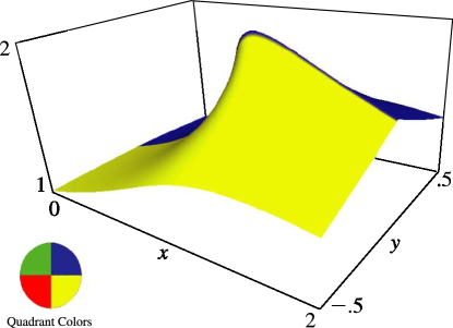
… ►In multivariate statistical analysis based on the multivariate normal distribution, the probability density functions of many random matrices are expressible in terms of generalized hypergeometric functions of matrix argument ${}_p{}^{}F_q^{}$, with $p\le 2$ and $q\le 1$. … ►For other statistical applications of ${}_p{}^{}F_q^{}$ functions of matrix argument see Perlman and Olkin (1980), Groeneboom and Truax (2000), Bhaumik and Sarkar (2002), Richards (2004) (monotonicity of power functions of multivariate statistical test criteria), Bingham et al. (1992) (Procrustes analysis), and Phillips (1986) (exact distributions of statistical test criteria). These references all use results related to the integral formulas (35.4.7) and (35.5.8). …

27: 8.17 Incomplete Beta Functions

… ►

8.17.7 $${\mathrm{B}}_x(a,b)=\frac{x^a}{a}F(a,1-b;a+1;x),$$

ⓘ

Symbols:

$F(a,b;c;z)$ or $F(\genfrac{}{}{0pt}{}{a,b}{c};z)$: $={}_2{}^{}F_1^{}(a,b;c;z)$ Gauss’ hypergeometric function, ${\mathrm{B}}_x(a,b)$: incomplete beta function, $a$: parameter, $b$: parameter and $x$: variable

A&S Ref:

6.6.8

Permalink:

http://dlmf.nist.gov/8.17.E7

Encodings:

pMML, png, TeX

See also:

Annotations for §8.17(ii), §8.17 and Ch.8

►

8.17.8 $${\mathrm{B}}_x(a,b)=\frac{x^a{(1-x)}^b}{a}F(a+b,1;a+1;x),$$

ⓘ

Symbols:

$F(a,b;c;z)$ or $F(\genfrac{}{}{0pt}{}{a,b}{c};z)$: $={}_2{}^{}F_1^{}(a,b;c;z)$ Gauss’ hypergeometric function, ${\mathrm{B}}_x(a,b)$: incomplete beta function, $a$: parameter, $b$: parameter and $x$: variable

Referenced by:

§8.17(i)

Permalink:

http://dlmf.nist.gov/8.17.E8

Encodings:

pMML, png, TeX

See also:

Annotations for §8.17(ii), §8.17 and Ch.8

►

8.17.9 $${\mathrm{B}}_x(a,b)=\frac{x^a{(1-x)}^{b-1}}{a}F(\genfrac{}{}{0pt}{}{1,1-b}{a+1};\frac{x}{x-1}).$$

ⓘ

Symbols:

$F(a,b;c;z)$ or $F(\genfrac{}{}{0pt}{}{a,b}{c};z)$: $={}_2{}^{}F_1^{}(a,b;c;z)$ Gauss’ hypergeometric function, ${\mathrm{B}}_x(a,b)$: incomplete beta function, $a$: parameter, $b$: parameter and $x$: variable

Referenced by:

§8.18(i)

Permalink:

http://dlmf.nist.gov/8.17.E9

Encodings:

pMML, png, TeX

See also:

Annotations for §8.17(ii), §8.17 and Ch.8

►For the hypergeometric function $F(a,b;c;z)$ see §15.2(i). … ►

8.17.24 $$I_x(m,n)={(1-x)}^n\sum _{j=m}^{\mathrm{\infty }}\left(\genfrac{}{}{0.0pt}{}{n+j-1}{j}\right)x^j,$$ $m,n$ positive integers; .

ⓘ

Symbols:

$I_x(a,b)$: incomplete beta function, $\left(\genfrac{}{}{0.0pt}{}{m}{n}\right)$: binomial coefficient, $n$: nonnegative integer and $x$: variable

A&S Ref:

26.5.26 (The upper limit of summation has been corrected.)

Referenced by:

§8.17(i), Erratum (V1.0.5) for Chapters 8, 20, 36

Permalink:

http://dlmf.nist.gov/8.17.E24

Encodings:

pMML, png, TeX

Addition (effective with 1.0.5):

This equation is the same as Equation (26.5.26) of Abramowitz and Stegun (1964), except that the upper limit of the summation has been corrected to $\mathrm{\infty }$.

Suggested 2011-03-23 by Stephen Bourn

See also:

Annotations for §8.17(vii), §8.17 and Ch.8

…

28: 15.1 Special Notation

… ►

15.1.1 $${}_2{}^{}F_1^{}(a,b;c;z)=F(a,b;c;z)=F(\genfrac{}{}{0pt}{}{a,b}{c};z),$$

ⓘ

Symbols:

$F(a,b;c;z)$ or $F(\genfrac{}{}{0pt}{}{a,b}{c};z)$: $={}_2{}^{}F_1^{}(a,b;c;z)$ Gauss’ hypergeometric function, ${}_2{}^{}F_1^{}(a,b;c;z)$: $=F(a,b;c;z)$ notation for Gauss’ hypergeometric function, $z$: complex variable, $a$: real or complex parameter, $b$: real or complex parameter and $c$: real or complex parameter

Permalink:

http://dlmf.nist.gov/15.1.E1

Encodings:

pMML, png, TeX

See also:

Annotations for §15.1 and Ch.15

… ►

15.1.2 $$\frac{F(a,b;c;z)}{\mathrm{\Gamma }\left(c\right)}=𝐅(a,b;c;z)=𝐅(\genfrac{}{}{0pt}{}{a,b}{c};z)={}_2{}^{}𝐅_1^{}(a,b;c;z),$$

ⓘ

Symbols:

$\mathrm{\Gamma }\left(z\right)$: gamma function, $F(a,b;c;z)$ or $F(\genfrac{}{}{0pt}{}{a,b}{c};z)$: $={}_2{}^{}F_1^{}(a,b;c;z)$ Gauss’ hypergeometric function, ${}_p{}^{}𝐅_q^{}(𝐚;𝐛;z)$ or ${}_p{}^{}𝐅_q^{}(\genfrac{}{}{0pt}{}{𝐚}{𝐛};z)$: scaled (or Olver’s) generalized hypergeometric function, $𝐅(a,b;c;z)$ or $𝐅(\genfrac{}{}{0pt}{}{a,b}{c};z)$: $={}_2{}^{}𝐅_1^{}(a,b;c;z)$ Olver’s hypergeometric function, $z$: complex variable, $a$: real or complex parameter, $b$: real or complex parameter and $c$: real or complex parameter

Permalink:

http://dlmf.nist.gov/15.1.E2

Encodings:

pMML, png, TeX

See also:

Annotations for §15.1 and Ch.15

…

29: 15.16 Products

… ►

15.16.1 $$F(\genfrac{}{}{0pt}{}{a,b}{c-\frac{1}{2}};z)F(\genfrac{}{}{0pt}{}{c-a,c-b}{c+\frac{1}{2}};z)=\sum _{s=0}^{\mathrm{\infty }}\frac{{\left(c\right)}_s}{{\left(c+\frac{1}{2}\right)}_s}{A}_s{z}^s,$$ ,

ⓘ

Symbols:

$F(a,b;c;z)$ or $F(\genfrac{}{}{0pt}{}{a,b}{c};z)$: $={}_2{}^{}F_1^{}(a,b;c;z)$ Gauss’ hypergeometric function, ${\left(a\right)}_n$: Pochhammer’s symbol (or shifted factorial), $s$: nonnegative integer, $z$: complex variable, $a$: real or complex parameter, $b$: real or complex parameter, $c$: real or complex parameter and $A_s$: coefficients

Permalink:

http://dlmf.nist.gov/15.16.E1

Encodings:

pMML, png, TeX

See also:

Annotations for §15.16 and Ch.15

… ►

15.16.2 $${(1-z)}^{a+b-c}F(2a,2b;2c-1;z)=\sum _{s=0}^{\mathrm{\infty }}{A}_s{z}^s,$$ .

ⓘ

Symbols:

$F(a,b;c;z)$ or $F(\genfrac{}{}{0pt}{}{a,b}{c};z)$: $={}_2{}^{}F_1^{}(a,b;c;z)$ Gauss’ hypergeometric function, $s$: nonnegative integer, $z$: complex variable, $a$: real or complex parameter, $b$: real or complex parameter, $c$: real or complex parameter and $A_s$: coefficients

Permalink:

http://dlmf.nist.gov/15.16.E2

Encodings:

pMML, png, TeX

See also:

Annotations for §15.16 and Ch.15

… ►

15.16.3 $$F(\genfrac{}{}{0pt}{}{a,b}{c};z)F(\genfrac{}{}{0pt}{}{a,b}{c};\zeta )=\sum _{s=0}^{\mathrm{\infty }}\frac{{\left(a\right)}_s{\left(b\right)}_s{\left(c-a\right)}_s{\left(c-b\right)}_s}{{\left(c\right)}_s{\left(c\right)}_{2s}s!}{\left(z\zeta \right)}^{s}F(\genfrac{}{}{0pt}{}{a+s,b+s}{c+2s};z+\zeta -z\zeta ),$$ , , .

ⓘ

Symbols:

$F(a,b;c;z)$ or $F(\genfrac{}{}{0pt}{}{a,b}{c};z)$: $={}_2{}^{}F_1^{}(a,b;c;z)$ Gauss’ hypergeometric function, ${\left(a\right)}_n$: Pochhammer’s symbol (or shifted factorial), $!$: factorial (as in $n!$), $s$: nonnegative integer, $z$: complex variable, $a$: real or complex parameter, $b$: real or complex parameter and $c$: real or complex parameter

Permalink:

http://dlmf.nist.gov/15.16.E3

Encodings:

pMML, png, TeX

See also:

Annotations for §15.16 and Ch.15

►

15.16.4 $$F(\genfrac{}{}{0pt}{}{a,b}{c};z)F(\genfrac{}{}{0pt}{}{-a,-b}{-c};z)+\frac{ab(a-c)(b-c)}{c^2(1-c^2)}{z}^{2}F(\genfrac{}{}{0pt}{}{1+a,1+b}{2+c};z)F(\genfrac{}{}{0pt}{}{1-a,1-b}{2-c};z)=1.$$

ⓘ

Symbols:

$F(a,b;c;z)$ or $F(\genfrac{}{}{0pt}{}{a,b}{c};z)$: $={}_2{}^{}F_1^{}(a,b;c;z)$ Gauss’ hypergeometric function, $z$: complex variable, $a$: real or complex parameter, $b$: real or complex parameter and $c$: real or complex parameter

Referenced by:

§15.16

Permalink:

http://dlmf.nist.gov/15.16.E4

Encodings:

pMML, png, TeX

See also:

Annotations for §15.16 and Ch.15

… ►

15.16.5 $$F(\genfrac{}{}{0pt}{}{\frac{1}{2}+\lambda ,-\frac{1}{2}-\nu }{1+\lambda +\mu };z)F(\genfrac{}{}{0pt}{}{\frac{1}{2}-\lambda ,\frac{1}{2}+\nu }{1+\nu +\mu };1-z)+F(\genfrac{}{}{0pt}{}{\frac{1}{2}+\lambda ,\frac{1}{2}-\nu }{1+\lambda +\mu };z)F(\genfrac{}{}{0pt}{}{-\frac{1}{2}-\lambda ,\frac{1}{2}+\nu }{1+\nu +\mu };1-z)-F(\genfrac{}{}{0pt}{}{\frac{1}{2}+\lambda ,\frac{1}{2}-\nu }{1+\lambda +\mu };z)F(\genfrac{}{}{0pt}{}{\frac{1}{2}-\lambda ,\frac{1}{2}+\nu }{1+\nu +\mu };1-z)=\frac{\mathrm{\Gamma }\left(1+\lambda +\mu \right)\mathrm{\Gamma }\left(1+\nu +\mu \right)}{\mathrm{\Gamma }\left(\lambda +\mu +\nu +\frac{3}{2}\right)\mathrm{\Gamma }\left(\frac{1}{2}+\nu \right)},$$ , .

ⓘ

Symbols:

$\mathrm{\Gamma }\left(z\right)$: gamma function, $F(a,b;c;z)$ or $F(\genfrac{}{}{0pt}{}{a,b}{c};z)$: $={}_2{}^{}F_1^{}(a,b;c;z)$ Gauss’ hypergeometric function, $\pi$: the ratio of the circumference of a circle to its diameter, $\mathrm{ph}$: phase and $z$: complex variable

Permalink:

http://dlmf.nist.gov/15.16.E5

Encodings:

pMML, png, TeX

See also:

Annotations for §15.16, §15.16 and Ch.15

…

30: 16.6 Transformations of Variable

… ►

16.6.1 $${}_3{}^{}F_2^{}(\genfrac{}{}{0pt}{}{a,b,c}{a-b+1,a-c+1};z)={(1-z)}^{-a}{}_3{}^{}F_2^{}(\genfrac{}{}{0pt}{}{a-b-c+1,\frac{1}{2}a,\frac{1}{2}(a+1)}{a-b+1,a-c+1};\frac{-4z}{{(1-z)}^2}).$$

ⓘ

Symbols:

${}_p{}^{}F_q^{}(a_1,\mathrm{\dots },a_p;b_1,\mathrm{\dots },b_q;z)$ or ${}_p{}^{}F_q^{}(\genfrac{}{}{0pt}{}{a_1,\mathrm{\dots },a_p}{b_1,\mathrm{\dots },b_q};z)$: alternatively ${}_p{}^{}F_q^{}(𝐚;𝐛;z)$ or ${}_p{}^{}F_q^{}(\genfrac{}{}{0pt}{}{𝐚}{𝐛};z)$
generalized hypergeometric function, $z$: complex variable, $a,a_1,\mathrm{\dots },a_p$: real or complex parameters and $b,b_1,\mathrm{\dots },b_q$: real or complex parameters

Referenced by:

§16.6

Permalink:

http://dlmf.nist.gov/16.6.E1

Encodings:

pMML, png, TeX

See also:

Annotations for §16.6, §16.6 and Ch.16

… ►

16.6.2 $${}_3{}^{}F_2^{}(\genfrac{}{}{0pt}{}{a,2b-a-1,2-2b+a}{b,a-b+\frac{3}{2}};\frac{z}{4})={(1-z)}^{-a}{}_3{}^{}F_2^{}(\genfrac{}{}{0pt}{}{\frac{1}{3}a,\frac{1}{3}a+\frac{1}{3},\frac{1}{3}a+\frac{2}{3}}{b,a-b+\frac{3}{2}};\frac{-27z}{4{(1-z)}^3}).$$

ⓘ

Symbols:

${}_p{}^{}F_q^{}(a_1,\mathrm{\dots },a_p;b_1,\mathrm{\dots },b_q;z)$ or ${}_p{}^{}F_q^{}(\genfrac{}{}{0pt}{}{a_1,\mathrm{\dots },a_p}{b_1,\mathrm{\dots },b_q};z)$: alternatively ${}_p{}^{}F_q^{}(𝐚;𝐛;z)$ or ${}_p{}^{}F_q^{}(\genfrac{}{}{0pt}{}{𝐚}{𝐛};z)$
generalized hypergeometric function, $z$: complex variable, $a,a_1,\mathrm{\dots },a_p$: real or complex parameters and $b,b_1,\mathrm{\dots },b_q$: real or complex parameters

Referenced by:

§16.6

Permalink:

http://dlmf.nist.gov/16.6.E2

Encodings:

pMML, png, TeX

See also:

Annotations for §16.6, §16.6 and Ch.16

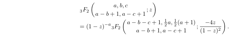
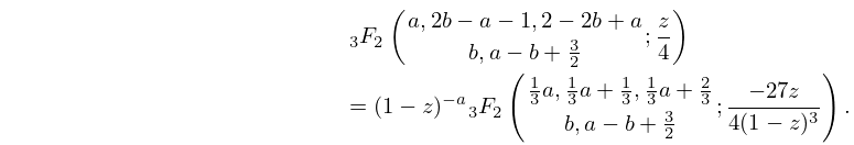
►For Kummer-type transformations of ${}_2{}^{}F_2^{}$ functions see Miller (2003) and Paris (2005a), and for further transformations see Erdélyi et al. (1953a, §4.5), Miller and Paris (2011), Choi and Rathie (2013) and Wang and Rathie (2013).