Fa%C3%A0%20di%20Bruno%20formula

SearchAdvancedHelp

(0.003 seconds)

21—30 of 308 matching pages

21: Bibliography

… ►

Exact linearization of a Painlevé transcendent. Phys. Rev. Lett. 38 (20), pp. 1103–1106.

ⓘ

External Links:

Document, MathReview (Mark Adler)

Referenced by:

§32.11(ii), §32.13(i), §32.13(ii), §32.13(iii), §32.5.

Encodings:

BibTeX

… ►

On the degrees of irreducible factors of higher order Bernoulli polynomials. Acta Arith. 62 (4), pp. 329–342.

ⓘ

External Links:

ISSN 0065-1036, Pdf, MathReview (L. Skula), ZentralBlatt

Referenced by:

§24.12(iii).

Encodings:

BibTeX

… ►

Application of the combined nonlinear-condensation transformation to problems in statistical analysis and theoretical physics. Comput. Phys. Comm. 150 (1), pp. 1–20.

ⓘ

Notes:

Includes algorithms for Lerch’s transcendent. C and Mathematica codes by Aksenov and Jentschura are available.

External Links:

Code, Document

Referenced by:

1st item.

Encodings:

BibTeX

… ►

Repeated integrals and derivatives of $K$ Bessel functions. SIAM J. Math. Anal. 20 (1), pp. 169–175.

ⓘ

External Links:

ISSN 0036-1410, Document, MathReview (A. Haimovici), ZentralBlatt

Referenced by:

§10.43(iii).

Encodings:

BibTeX

… ►

Umbral calculus, Bailey chains, and pentagonal number theorems. J. Combin. Theory Ser. A 91 (1-2), pp. 464–475.

ⓘ

Notes:

In memory of Gian-Carlo Rota

External Links:

ISSN 0097-3165, Document, MathReview (Alessandro Di Bucchianico), ZentralBlatt

Referenced by:

§17.12.

Encodings:

BibTeX

…

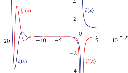
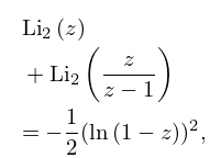
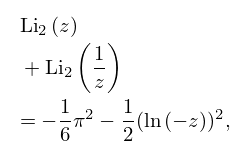
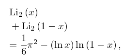
22: 25.12 Polylogarithms

… ►

25.12.3 $${\mathrm{Li}}_2\left(z\right)+{\mathrm{Li}}_2\left(\frac{z}{z-1}\right)=-\frac{1}{2}{(\ln \left(1-z\right))}^2,$$ $z\in ℂ\setminus [1,\mathrm{\infty })$.

ⓘ

Symbols:

$[a,b)$: half-closed interval, $ℂ$: complex plane, ${\mathrm{Li}}_2\left(z\right)$: dilogarithm, $\in$: element of, $\ln z$: principal branch of logarithm function, $\setminus$: set subtraction, $x$: real variable and $z$: complex variable

Keywords:

connection formula

Source:

Maximon (2003, (3.4), p. 2808)

A&S Ref:

27.7.5 (is a modified form with $z=1-x$)

Permalink:

http://dlmf.nist.gov/25.12.E3

Encodings:

pMML, png, TeX

See also:

Annotations for §25.12(i), §25.12 and Ch.25

►

25.12.4 $${\mathrm{Li}}_2\left(z\right)+{\mathrm{Li}}_2\left(\frac{1}{z}\right)=-\frac{1}{6}{\pi }^2-\frac{1}{2}{(\ln \left(-z\right))}^2,$$ $z\in ℂ\setminus [0,\mathrm{\infty })$.

ⓘ

Symbols:

$\pi$: the ratio of the circumference of a circle to its diameter, $[a,b)$: half-closed interval, $ℂ$: complex plane, ${\mathrm{Li}}_2\left(z\right)$: dilogarithm, $\in$: element of, $\ln z$: principal branch of logarithm function, $\setminus$: set subtraction and $z$: complex variable

Keywords:

connection formula

Source:

Maximon (2003, (3.2), p. 2808)

Referenced by:

§25.12(ii)

Permalink:

http://dlmf.nist.gov/25.12.E4

Encodings:

pMML, png, TeX

See also:

Annotations for §25.12(i), §25.12 and Ch.25

… ►

25.12.6 $${\mathrm{Li}}_2\left(x\right)+{\mathrm{Li}}_2\left(1-x\right)=\frac{1}{6}{\pi }^2-(\ln x)\ln \left(1-x\right),$$ .

ⓘ

Symbols:

$\pi$: the ratio of the circumference of a circle to its diameter, ${\mathrm{Li}}_2\left(z\right)$: dilogarithm, $\ln z$: principal branch of logarithm function and $x$: real variable

Keywords:

connection formula

Source:

Maximon (2003, (3.3), p. 2808)

Permalink:

http://dlmf.nist.gov/25.12.E6

Encodings:

pMML, png, TeX

See also:

Annotations for §25.12(i), §25.12 and Ch.25

… ►

►►

Figure 25.12.1: Dilogarithm function ${\mathrm{Li}}_2\left(x\right)$, Magnify

►

►

►

Figure 25.12.2: Absolute value of the dilogarithm function $\left|{\mathrm{Li}}_2\left(x+\mathrm{i}y\right)\right|$, $-20\le x\le 20$, $-20\le y\le 20$. … Magnify 3D Help

…

23: 6.20 Approximations

… ►

Cody and Thacher (1968) provides minimax rational approximations for $E_1\left(x\right)$, with accuracies up to 20S.

►

Cody and Thacher (1969) provides minimax rational approximations for $\mathrm{Ei}\left(x\right)$, with accuracies up to 20S.

►

MacLeod (1996b) provides rational approximations for the sine and cosine integrals and for the auxiliary functions $\mathrm{f}$ and $\mathrm{g}$, with accuracies up to 20S.

…

24: 13.30 Tables

… ►

Zhang and Jin (1996, pp. 411–423) tabulates $M(a,b,x)$ and $U(a,b,x)$ for $a=-5(.5)5$, $b=0.5(.5)5$, and $x=0.1,1,5,10,20,30$, 8S (for $M(a,b,x)$) and 7S (for $U(a,b,x)$).

…

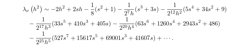
25: 28.16 Asymptotic Expansions for Large $q$

… ►

28.16.1 $${\lambda }_{\nu }\left(h^2\right)\sim -2h^2+2sh-\frac{1}{8}(s^2+1)-\frac{1}{2^{7}h}(s^3+3s)-\frac{1}{2^{12}{h}^2}(5s^4+34s^2+9)-\frac{1}{2^{17}{h}^3}(33s^5+410s^3+405s)-\frac{1}{2^{20}{h}^4}(63s^6+1260s^4+2943s^2+486)-\frac{1}{2^{25}{h}^5}(527s^7+15617s^5+69001s^3+41607s)+\mathrm{\cdots }.$$

ⓘ

Symbols:

${\lambda }_{\nu +2n}\left(q\right)$: eigenvalues of Mathieu equation, $\sim$: Poincaré asymptotic expansion, $h$: parameter and $\nu$: complex parameter

Permalink:

http://dlmf.nist.gov/28.16.E1

Encodings:

pMML, png, TeX

See also:

Annotations for §28.16 and Ch.28

…

26: Bibliography Z

… ►

Sul calcolo numerico della funzione di Struve ${𝐇}_{\nu }(z)$ . Rend. Sem. Mat. Univ. e Politec. Torino 32, pp. 251–269 (Italian. English summary).

ⓘ

External Links:

MathReview (Walter Gautschi), ZentralBlatt

Referenced by:

§11.13(i), 4th item.

Encodings:

BibTeX

►

Integrali di funzioni di Anger, Weber ed Airy-Hardy. Rend. Sem. Mat. Univ. Padova 58, pp. 275–285 (Italian).

ⓘ

External Links:

FullText, MathReview (M. E. Muldoon), ZentralBlatt

Referenced by:

§11.10(x).

Encodings:

BibTeX

►

Su un integrale definito del prodotto di due funzioni di Struve. Atti Accad. Sci. Torino Cl. Sci. Fis. Mat. Natur. 112 (1-2), pp. 63–81 (Italian).

ⓘ

External Links:

ISSN 0001-4419, MathReview, ZentralBlatt

Referenced by:

§11.7(ii).

Encodings:

BibTeX

… ►

Approximations to -, di- and tri-logarithms. J. Comput. Appl. Math. 202 (2), pp. 450–459.

ⓘ

External Links:

ISSN 0377-0427, Document, FullText, MathReview (F. Beukers), ZentralBlatt

Referenced by:

§25.18(i), §25.18(i).

Encodings:

BibTeX

… ►

Tables and formulae for the spherical functions $P_{-1/2+i\tau }^m(z)$ . Translated by E. L. Albasiny, Pergamon Press, Oxford.

ⓘ

Notes:

Translation of Žurina and Karmazina, Tablitsy i formuly dlya sfericheskikh funktsii $P_{-1/2+i\tau }^m(z)$ , Vyčisl. Centr Akad Nauk SSSR, Moscow. 1962

External Links:

MathReview, ZentralBlatt

Referenced by:

§14.20(vii).

Encodings:

BibTeX

…

27: 28.35 Tables

… ►

Blanch and Clemm (1965) includes values of ${\mathrm{Mc}}_n^{(2)}(x,\sqrt{q})$, $\mathrm{Mc}_n^{(2)}{}_{}{}^{\prime }(x,\sqrt{q})$ for $n=0(1)7$, $x=0(.02)1$; $n=8(1)15$, $x=0(.01)1$. Also ${\mathrm{Ms}}_n^{(2)}(x,\sqrt{q})$, $\mathrm{Ms}_n^{(2)}{}_{}{}^{\prime }(x,\sqrt{q})$ for $n=1(1)7$, $x=0(.02)1$; $n=8(1)15$, $x=0(.01)1$. In all cases $q=0(.05)1$. Precision is generally 7D. Approximate formulas and graphs are also included.

… ►

Ince (1932) includes eigenvalues $a_n$, $b_n$, and Fourier coefficients for $n=0$ or $1(1)6$, $q=0(1)10(2)20(4)40$; 7D. Also ${\mathrm{ce}}_n(x,q)$, ${\mathrm{se}}_n(x,q)$ for $q=0(1)10$, $x=1(1)90$, corresponding to the eigenvalues in the tables; 5D. Notation: $a_n={\mathrm{𝑏𝑒}}_n-2q$, $b_n={\mathrm{𝑏𝑜}}_n-2q$.

►

Kirkpatrick (1960) contains tables of the modified functions ${\mathrm{Ce}}_n(x,q)$, ${\mathrm{Se}}_{n+1}(x,q)$ for $n=0(1)5$, $q=1(1)20$, $x=0.1(.1)1$; 4D or 5D.

►

National Bureau of Standards (1967) includes the eigenvalues $a_n\left(q\right)$, $b_n\left(q\right)$ for $n=0(1)3$ with $q=0(.2)20(.5)37(1)100$, and $n=4(1)15$ with $q=0(2)100$; Fourier coefficients for ${\mathrm{ce}}_n(x,q)$ and ${\mathrm{se}}_n(x,q)$ for $n=0(1)15$, $n=1(1)15$, respectively, and various values of $q$ in the interval $[0,100]$; joining factors $g_{e,n}(\sqrt{q})$, $f_{e,n}(\sqrt{q})$ for $n=0(1)15$ with $q=0(.5\text{ to }10)100$ (but in a different notation). Also, eigenvalues for large values of $q$. Precision is generally 8D.

… ►

Zhang and Jin (1996, pp. 521–532) includes the eigenvalues $a_n\left(q\right)$, $b_{n+1}\left(q\right)$ for $n=0(1)4$, $q=0(1)50$; $n=0(1)20$ ($a$’s) or 19 ($b$’s), $q=1,3,5,10,15,25,50(50)200$. Fourier coefficients for ${\mathrm{ce}}_n(x,10)$, ${\mathrm{se}}_{n+1}(x,10)$, $n=0(1)7$. Mathieu functions ${\mathrm{ce}}_n(x,10)$, ${\mathrm{se}}_{n+1}(x,10)$, and their first $x$-derivatives for $n=0(1)4$, $x=0(5^{\circ }){90}^{\circ }$. Modified Mathieu functions ${\mathrm{Mc}}_n^{(j)}(x,\sqrt{10})$, ${\mathrm{Ms}}_{n+1}^{(j)}(x,\sqrt{10})$, and their first $x$-derivatives for $n=0(1)4$, $j=1,2$, $x=0(.2)4$. Precision is mostly 9S.

…

28: 7.24 Approximations

… ►

Cody (1969) provides minimax rational approximations for $\mathrm{erf}x$ and $\mathrm{erfc}x$. The maximum relative precision is about 20S.

… ►

Cody et al. (1970) gives minimax rational approximations to Dawson’s integral $F\left(x\right)$ (maximum relative precision 20S–22S).

…

29: 25.3 Graphics

… ►

►►

Figure 25.3.1: Riemann zeta function $\zeta \left(x\right)$ and its derivative ${\zeta }^{\prime }\left(x\right)$, $-20\le x\le 10$. Magnify

…

30: 27.2 Functions

… ►Euclid’s Elements (Euclid (1908, Book IX, Proposition 20)) gives an elegant proof that there are infinitely many primes. … ►

Table 27.2.2: Functions related to division.

► ►►►►►►

$n$	$\varphi \left(n\right)$	$d\left(n\right)$	$\sigma \left(n\right)$	$n$	$\varphi \left(n\right)$	$d\left(n\right)$	$\sigma \left(n\right)$	$n$	$\varphi \left(n\right)$	$d\left(n\right)$	$\sigma \left(n\right)$	$n$	$\varphi \left(n\right)$	$d\left(n\right)$	$\sigma \left(n\right)$
…
5	4	2	6	18	6	6	39	31	30	2	32	44	20	6	84
6	2	4	12	19	18	2	20	32	16	6	63	45	24	6	78
7	6	2	8	20	8	6	42	33	20	4	48	46	22	4	72
…
11	10	2	12	24	8	8	60	37	36	2	38	50	20	6	93
…

►