Barrett’s

SearchAdvancedHelp

(0.002 seconds)

31—40 of 602 matching pages

31: 25.19 Tables

… ►

Abramowitz and Stegun (1964) tabulates: $\zeta \left(n\right)$, $n=2,3,4,\mathrm{\dots }$, 20D (p. 811); ${\mathrm{Li}}_2\left(1-x\right)$, $x=0(.01)0.5$, 9D (p. 1005); $f(\theta )$, $\theta ={15}^{\circ }(1^{\circ }){30}^{\circ }(2^{\circ }){90}^{\circ }(5^{\circ }){180}^{\circ }$, $f(\theta )+\theta \ln \theta$, $\theta =0(1^{\circ }){15}^{\circ }$, 6D (p. 1006). Here $f(\theta )$ denotes Clausen’s integral, given by the right-hand side of (25.12.9).

… ►

Cloutman (1989) tabulates $\mathrm{\Gamma }\left(s+1\right)F_s(x)$, where $F_s(x)$ is the Fermi–Dirac integral (25.12.14), for $s=-\frac{1}{2},\frac{1}{2},\frac{3}{2},\frac{5}{2}$, $x=-5(.05)25$, to 12S.

►

Fletcher et al. (1962, §22.1) lists many sources for earlier tables of $\zeta \left(s\right)$ for both real and complex $s$. §22.133 gives sources for numerical values of coefficients in the Riemann–Siegel formula, §22.15 describes tables of values of $\zeta (s,a)$, and §22.17 lists tables for some Dirichlet $L$-functions for real characters. For tables of dilogarithms, polylogarithms, and Clausen’s integral see §§22.84–22.858.

32: 13.11 Series

… ►

13.11.1 $$M(a,b,z)=\mathrm{\Gamma }\left(a-\frac{1}{2}\right){\mathrm{e}}^{\frac{1}{2}z}{\left(\frac{1}{4}z\right)}^{\frac{1}{2}-a}\sum _{s=0}^{\mathrm{\infty }}\frac{{\left(2a-1\right)}_s{\left(2a-b\right)}_s}{{\left(b\right)}_{s}s!}\left(a-\frac{1}{2}+s\right)I_{a-\frac{1}{2}+s}\left(\frac{1}{2}z\right),$$ $a+\frac{1}{2},b\ne 0,-1,-2,\mathrm{\dots }$,

ⓘ

Symbols:

$\mathrm{\Gamma }\left(z\right)$: gamma function, $M(a,b,z)$: $={}_1{}^{}F_1^{}(a;b;z)$ Kummer confluent hypergeometric function, ${\left(a\right)}_n$: Pochhammer’s symbol (or shifted factorial), $\mathrm{e}$: base of natural logarithm, $!$: factorial (as in $n!$), $I_{\nu }\left(z\right)$: modified Bessel function of the first kind, $s$: nonnegative integer and $z$: complex variable

Referenced by:

§13.6(iii), §13.6(iii), §8.7

Permalink:

http://dlmf.nist.gov/13.11.E1

Encodings:

pMML, png, TeX

See also:

Annotations for §13.11 and Ch.13

►

13.11.2 $$M(a,b,z)=\mathrm{\Gamma }\left(b-a-\frac{1}{2}\right){\mathrm{e}}^{\frac{1}{2}z}{\left(\frac{1}{4}z\right)}^{a-b+\frac{1}{2}}\sum _{s=0}^{\mathrm{\infty }}{(-1)}^s\frac{{\left(2b-2a-1\right)}_s{\left(b-2a\right)}_s(b-a-\frac{1}{2}+s)}{{\left(b\right)}_{s}s!}{I}_{b-a-\frac{1}{2}+s}\left(\frac{1}{2}z\right),$$ $b-a+\frac{1}{2},b\ne 0,-1,-2,\mathrm{\dots }$.

ⓘ

Symbols:

$\mathrm{\Gamma }\left(z\right)$: gamma function, $M(a,b,z)$: $={}_1{}^{}F_1^{}(a;b;z)$ Kummer confluent hypergeometric function, ${\left(a\right)}_n$: Pochhammer’s symbol (or shifted factorial), $\mathrm{e}$: base of natural logarithm, $!$: factorial (as in $n!$), $I_{\nu }\left(z\right)$: modified Bessel function of the first kind, $s$: nonnegative integer and $z$: complex variable

Proof sketch:

Combine (13.24.1) with (13.14.4).

A&S Ref:

13.3.6

Referenced by:

§13.11, §13.6(iii), §13.6(iii), Erratum (V1.1.0) for Additions

Permalink:

http://dlmf.nist.gov/13.11.E2

Encodings:

pMML, png, TeX

Addition (effective with 1.1.0):

This equation was added.

See also:

Annotations for §13.11 and Ch.13

… ►

13.11.3 $$𝐌(a,b,z)={\mathrm{e}}^{\frac{1}{2}z}\sum _{s=0}^{\mathrm{\infty }}{A}_s{\left(b-2a\right)}^{\frac{1}{2}(1-b-s)}{\left(\frac{1}{2}z\right)}^{\frac{1}{2}(1-b+s)}{J}_{b-1+s}\left(\sqrt{2z(b-2a)}\right),$$

ⓘ

Symbols:

$J_{\nu }\left(z\right)$: Bessel function of the first kind, $𝐌(a,b,z)$: Olver’s confluent hypergeometric function, $\mathrm{e}$: base of natural logarithm, $s$: nonnegative integer, $z$: complex variable and $A_n$: coefficients

Source:

Slater (1960, §3.8)

A&S Ref:

13.3.7

Referenced by:

§13.11, Erratum (V1.1.0) for Additions

Permalink:

http://dlmf.nist.gov/13.11.E3

Encodings:

pMML, png, TeX

Addition (effective with 1.1.0):

This equation was added.

See also:

Annotations for §13.11 and Ch.13

…

33: 12.9 Asymptotic Expansions for Large Variable

… ►

12.9.1 $$U(a,z)\sim {\mathrm{e}}^{-\frac{1}{4}{z}^2}{z}^{-a-\frac{1}{2}}\sum _{s=0}^{\mathrm{\infty }}{(-1)}^s\frac{{\left(\frac{1}{2}+a\right)}_{2s}}{s!{(2z^2)}^s},$$ ,

ⓘ

Symbols:

${\left(a\right)}_n$: Pochhammer’s symbol (or shifted factorial), $\sim$: Poincaré asymptotic expansion, $\pi$: the ratio of the circumference of a circle to its diameter, $\mathrm{e}$: base of natural logarithm, $!$: factorial (as in $n!$), $U(a,z)$: parabolic cylinder function, $\mathrm{ph}$: phase, $z$: complex variable, $s$: nonnegative integer, $a$: real or complex parameter and $\delta$: arbitrary small positive constant

A&S Ref:

19.8.1 (modification of)

Referenced by:

§12.9(i), §12.9(ii)

Permalink:

http://dlmf.nist.gov/12.9.E1

Encodings:

pMML, png, TeX

See also:

Annotations for §12.9(i), §12.9 and Ch.12

►

12.9.2 $$V(a,z)\sim \sqrt{\frac{2}{\pi }}{\mathrm{e}}^{\frac{1}{4}{z}^2}{z}^{a-\frac{1}{2}}\sum _{s=0}^{\mathrm{\infty }}\frac{{\left(\frac{1}{2}-a\right)}_{2s}}{s!{(2z^2)}^s},$$ .

ⓘ

Symbols:

${\left(a\right)}_n$: Pochhammer’s symbol (or shifted factorial), $\sim$: Poincaré asymptotic expansion, $\pi$: the ratio of the circumference of a circle to its diameter, $\mathrm{e}$: base of natural logarithm, $!$: factorial (as in $n!$), $V(a,z)$: parabolic cylinder function, $\mathrm{ph}$: phase, $z$: complex variable, $s$: nonnegative integer, $a$: real or complex parameter and $\delta$: arbitrary small positive constant

A&S Ref:

19.8.2 (modification of)

Referenced by:

§12.9(i), §12.9(ii)

Permalink:

http://dlmf.nist.gov/12.9.E2

Encodings:

pMML, png, TeX

See also:

Annotations for §12.9(i), §12.9 and Ch.12

►

12.9.3 $$U(a,z)\sim {\mathrm{e}}^{-\frac{1}{4}{z}^2}{z}^{-a-\frac{1}{2}}\sum _{s=0}^{\mathrm{\infty }}{(-1)}^s\frac{{\left(\frac{1}{2}+a\right)}_{2s}}{s!{(2z^2)}^s}\pm \mathrm{i}\frac{\sqrt{2\pi }}{\mathrm{\Gamma }\left(\frac{1}{2}+a\right)}{\mathrm{e}}^{\mp \mathrm{i}\pi a}{\mathrm{e}}^{\frac{1}{4}{z}^2}{z}^{a-\frac{1}{2}}\sum _{s=0}^{\mathrm{\infty }}\frac{{\left(\frac{1}{2}-a\right)}_{2s}}{s!{(2z^2)}^s},$$ $\frac{1}{4}\pi +\delta \le \pm \mathrm{ph}z\le \frac{5}{4}\pi -\delta$ ,

ⓘ

Symbols:

$\mathrm{\Gamma }\left(z\right)$: gamma function, ${\left(a\right)}_n$: Pochhammer’s symbol (or shifted factorial), $\sim$: Poincaré asymptotic expansion, $\pi$: the ratio of the circumference of a circle to its diameter, $\mathrm{e}$: base of natural logarithm, $!$: factorial (as in $n!$), $\mathrm{i}$: imaginary unit, $U(a,z)$: parabolic cylinder function, $\mathrm{ph}$: phase, $z$: complex variable, $s$: nonnegative integer, $a$: real or complex parameter and $\delta$: arbitrary small positive constant

Permalink:

http://dlmf.nist.gov/12.9.E3

Encodings:

pMML, png, TeX

See also:

Annotations for §12.9(i), §12.9 and Ch.12

►

12.9.4 $$V(a,z)\sim \sqrt{\frac{2}{\pi }}{\mathrm{e}}^{\frac{1}{4}{z}^2}{z}^{a-\frac{1}{2}}\sum _{s=0}^{\mathrm{\infty }}\frac{{\left(\frac{1}{2}-a\right)}_{2s}}{s!{(2z^2)}^s}\pm \frac{\mathrm{i}}{\mathrm{\Gamma }\left(\frac{1}{2}-a\right)}{\mathrm{e}}^{-\frac{1}{4}{z}^2}{z}^{-a-\frac{1}{2}}\sum _{s=0}^{\mathrm{\infty }}{(-1)}^s\frac{{\left(\frac{1}{2}+a\right)}_{2s}}{s!{(2z^2)}^s},$$ $-\frac{1}{4}\pi +\delta \le \pm \mathrm{ph}z\le \frac{3}{4}\pi -\delta$.

ⓘ

Symbols:

$\mathrm{\Gamma }\left(z\right)$: gamma function, ${\left(a\right)}_n$: Pochhammer’s symbol (or shifted factorial), $\sim$: Poincaré asymptotic expansion, $\pi$: the ratio of the circumference of a circle to its diameter, $\mathrm{e}$: base of natural logarithm, $!$: factorial (as in $n!$), $\mathrm{i}$: imaginary unit, $V(a,z)$: parabolic cylinder function, $\mathrm{ph}$: phase, $z$: complex variable, $s$: nonnegative integer, $a$: real or complex parameter and $\delta$: arbitrary small positive constant

Referenced by:

§12.9(i)

Permalink:

http://dlmf.nist.gov/12.9.E4

Encodings:

pMML, png, TeX

See also:

Annotations for §12.9(i), §12.9 and Ch.12

…

34: 21.1 Special Notation

… ► ►►►►►►

$g,h$	positive integers.
…
$S^g$	set of $g$-dimensional vectors with elements in $S$.
$|S|$	number of elements of the set $S$.
$S_1{S}_2$	set of all elements of the form “$\text{element of }{S}_1\times \text{element of }{S}_2$”.
$S_1/S_2$	set of all elements of $S_1$, modulo elements of $S_2$. Thus two elements of $S_1/S_2$ are equivalent if they are both in $S_1$ and their difference is in $S_2$. (For an example see §20.12(ii).)
…

…

35: 3.9 Acceleration of Convergence

… ►

§3.9(ii) Euler’s Transformation of Series

… ►Euler’s transformation is usually applied to alternating series. … ►

§3.9(iii) Aitken’s ${\mathrm{\Delta }}^2$-Process

… ►

§3.9(v) Levin’s and Weniger’s Transformations

►We give a special form of Levin’s transformation in which the sequence $s=\{s_n\}$ of partial sums $s_n={\sum }_{j=0}^n{a}_j$ is transformed into: …

36: 25.11 Hurwitz Zeta Function

… ► $\zeta (s,a)$ has a meromorphic continuation in the $s$-plane, its only singularity in $ℂ$ being a simple pole at $s=1$ with residue $1$. … ►

$s$-Derivatives

►In (25.11.18)–(25.11.24) primes on $\zeta$ denote derivatives with respect to $s$. … ►where $G$ is Catalan’s constant: … ►As $\beta \to \pm \mathrm{\infty }$ with $s$ fixed, $\mathrm{\Re }s>1$, …

37: 7.16 Generalized Error Functions

§7.16 Generalized Error Functions

►Generalizations of the error function and Dawson’s integral are ${\int }_0^x{\mathrm{e}}^{-t^p}dt$ and ${\int }_0^x{\mathrm{e}}^{t^p}dt$. …

38: 17.5 ${}_0{}^{}\varphi _0^{},{}_1{}^{}\varphi _0^{},{}_1{}^{}\varphi _1^{}$ Functions

… ►

Euler’s Second Sum

… ►

17.5.2 $${}_1{}^{}\varphi _0^{}(a;-;q,z)=\frac{{(az;q)}_{\mathrm{\infty }}}{{(z;q)}_{\mathrm{\infty }}},$$ ;

ⓘ

Symbols:

${(a;q)}_n$: $q$-Pochhammer symbol (or $q$-shifted factorial), ${}_{r+1}{}^{}\varphi _s^{}(a_0,\mathrm{\dots },a_r;b_1,\mathrm{\dots },b_s;q,z)$ or ${}_{r+1}{}^{}\varphi _s^{}(\genfrac{}{}{0pt}{}{a_0,\mathrm{\dots },a_r}{b_1,\mathrm{\dots },b_s};q,z)$: basic hypergeometric (or $q$-hypergeometric) function, $q$: complex base and $z$: complex variable

Permalink:

http://dlmf.nist.gov/17.5.E2

Encodings:

pMML, png, TeX

See also:

Annotations for §17.5, §17.5 and Ch.17

… ►

17.5.3 $${}_1{}^{}\varphi _0^{}(q^{-n};-;q,z)={(z{q}^{-n};q)}_n.$$

ⓘ

Symbols:

${(a;q)}_n$: $q$-Pochhammer symbol (or $q$-shifted factorial), ${}_{r+1}{}^{}\varphi _s^{}(a_0,\mathrm{\dots },a_r;b_1,\mathrm{\dots },b_s;q,z)$ or ${}_{r+1}{}^{}\varphi _s^{}(\genfrac{}{}{0pt}{}{a_0,\mathrm{\dots },a_r}{b_1,\mathrm{\dots },b_s};q,z)$: basic hypergeometric (or $q$-hypergeometric) function, $q$: complex base, $n$: nonnegative integer and $z$: complex variable

Permalink:

http://dlmf.nist.gov/17.5.E3

Encodings:

pMML, png, TeX

See also:

Annotations for §17.5, §17.5 and Ch.17

… ►

Euler’s First Sum

… ►

Cauchy’s Sum

…

39: 30.11 Radial Spheroidal Wave Functions

… ►

$S_n^{m(3)}(z,\gamma )=S_n^{m(1)}(z,\gamma )+\mathrm{i}{S}_n^{m(2)}(z,\gamma ),$

►

$S_n^{m(4)}(z,\gamma )=S_n^{m(1)}(z,\gamma )-\mathrm{i}{S}_n^{m(2)}(z,\gamma ).$

… ►

►►

Figure 30.11.1: $S_n^{0(1)}(x,2)$, $n=0,1$, $1\le x\le 10$. Magnify

►

►►

Figure 30.11.2: $S_n^{0(1)}(\mathrm{i}y,2\mathrm{i})$, $n=0,1$, $0\le y\le 10$. Magnify

►

►►

Figure 30.11.3: $S_n^{1(1)}(x,2)$, $n=1,2$, $1\le x\le 10$. Magnify

…

40: 12.11 Zeros

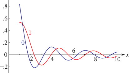
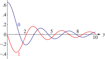
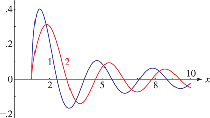
… ►When $a>-\frac{1}{2}$ the zeros are asymptotically given by $z_{a,s}$ and $\overline{z_{a,s}}$, where $s$ is a large positive integer and … ►Numerical calculations in this case show that $z_{\frac{1}{2},s}$ corresponds to the $s$th zero on the string; compare §7.13(ii). … ►For example, let the $s$th real zeros of $U(a,x)$ and $U^{\prime }(a,x)$, counted in descending order away from the point $z=2\sqrt{-a}$, be denoted by $u_{a,s}$ and $u_{a,s}^{\prime }$, respectively. …Here $\alpha ={\mu }^{-\frac{4}{3}}{a}_s$, $a_s$ denoting the $s$th negative zero of the function $\mathrm{Ai}$ (see §9.9(i)). … ►where $\beta ={\mu }^{-\frac{4}{3}}{a}_s^{\prime }$, $a_s^{\prime }$ denoting the $s$th negative zero of the function ${\mathrm{Ai}}^{\prime }$ and …