Appell%0Afunctions
(0.001 seconds)
21—30 of 701 matching pages
21: 24.2 Definitions and Generating Functions
22: 11.14 Tables
Abramowitz and Stegun (1964, Chapter 12) tabulates , , and for and , to 6D or 7D.
Agrest et al. (1982) tabulates and for and to 11D.
Abramowitz and Stegun (1964, Chapter 12) tabulates and for to 5D or 7D; , , and for to 6D.
Agrest et al. (1982) tabulates and for to 11D.
Agrest and Maksimov (1971, Chapter 11) defines incomplete Struve, Anger, and Weber functions and includes tables of an incomplete Struve function for , , and , together with surface plots.
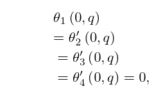
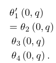
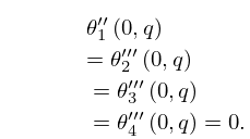
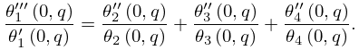
23: 20.4 Values at = 0
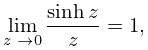
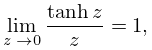
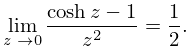
24: 4.31 Special Values and Limits
25: 32.4 Isomonodromy Problems
26: 14.33 Tables
Abramowitz and Stegun (1964, Chapter 8) tabulates for , , 5–8D; for , , 5–7D; and for , , 6–8D; and for , , 6S; and for , , 6S. (Here primes denote derivatives with respect to .)
Zhang and Jin (1996, Chapter 4) tabulates for , , 7D; for , , 8D; for , , 8S; for , , 8D; for , , , , 8S; for , , 8S; for , , , 5D; for , , 7S; for , , 8S. Corresponding values of the derivative of each function are also included, as are 6D values of the first 5 -zeros of and of its derivative for , .
Belousov (1962) tabulates (normalized) for , , , 6D.
Žurina and Karmazina (1963) tabulates the conical functions for , , 7S; for , , 7S. Auxiliary tables are included to assist computation for larger values of when .
27: 15.15 Sums
28: 11.15 Approximations
Luke (1975, pp. 416–421) gives Chebyshev-series expansions for , , , and , , for ; , , , and , , ; the coefficients are to 20D.
MacLeod (1993) gives Chebyshev-series expansions for , , , and , , ; the coefficients are to 20D.
Newman (1984) gives polynomial approximations for for , , and rational-fraction approximations for for , . The maximum errors do not exceed 1.2×10⁻⁸ for the former and 2.5×10⁻⁸ for the latter.
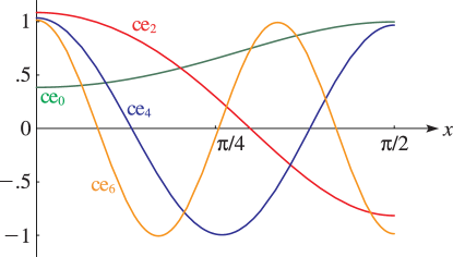
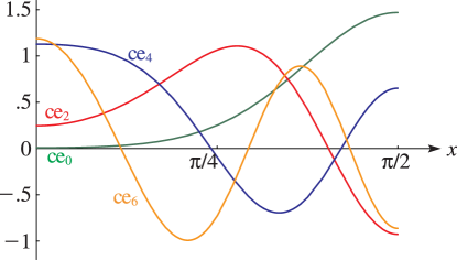
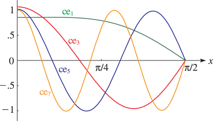
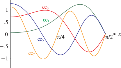
29: 28.3 Graphics
 ►
►
 ►
►
 ►
►
 ►
►
