…
►Let
be an arbitrary integer, and
and
denote the branches obtained from the principal branches by making
circuits, in the positive sense, of the ellipse having
as foci and passing through
.
…
►Next, let
and
denote the branches obtained from the principal branches by encircling the branch point
(but not the branch point
)
times in the positive sense.
…the limiting value being taken in (
14.24.4) when
.
►For fixed
, other than
or
, each branch of
and
is an entire function of each parameter
and
.
►The behavior of
and
as
from the left on the upper or lower side of the cut from
to
can be deduced from (
14.8.7)–(
14.8.11), combined with (
14.24.1) and (
14.24.2) with
.
…
►The principal values of
and
(§
14.21(i)) are given by
►
14.25.1
,
►
14.25.2
,
…
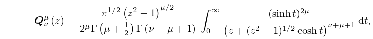
►For corresponding contour integrals, with less restrictions on
and
, see
Olver (1997b, pp. 174–179), and for further integral representations see
Magnus et al. (1966, §4.6.1).
…
►
14.14.1
…
►
►
…
►
14.14.3
,
…
►
…
…
►
exists for all values of
and
.
is undefined when
.
►When
, (
14.3.1) reduces to
…
►When
, (
14.3.6) reduces to
…
►As standard solutions of (
14.2.2) we take the pair
and
, where
…
…
►except that
does not exist when
.
…
►The
principal branches correspond to the principal branches of the functions
and
on the right-hand sides of the equations (
13.14.2) and (
13.14.3); compare §
4.2(i).
…
►Except when
, each branch of the functions
and
is entire in
and
.
…
►When
is an integer we may use the results of §
13.2(v) with the substitutions
,
, and
, where
is the solution of (
13.14.1) corresponding to the solution
of (
13.2.1).
…
►When
is not an integer
…
…
►For expansions of arbitrary functions in series of
functions see
Schäfke (1961b).
…
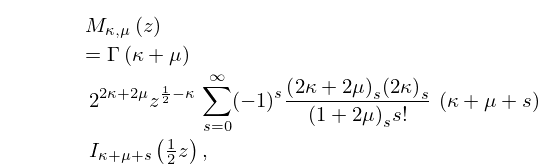
►
13.24.1
,
…
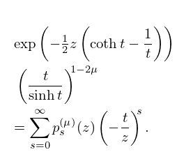
►
13.24.2
►where
,
, and higher polynomials
are defined by
►
13.24.3
…
…
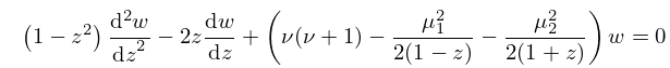
►
14.29.1
…
►As in the case of (
14.21.1), the solutions are hypergeometric functions, and (
14.29.1) reduces to (
14.21.1) when
.
…
…
►
§13.21(i) Large , Fixed
…
►When
through positive real values with
(
) fixed
…
►Other types of approximations when
through positive real values with
(
) fixed are as follows.
…
►
§13.21(ii) Large ,
…
►For the functions
,
,
, and
see §
10.2(ii), and for the
functions associated with
and
see §
2.8(iv).
…
…
►If
such that
, then
…
►
►
…
►If
such that
, then
…
►
…
…
►In this subsection see §§
10.2(ii),
10.25(ii) for the functions
,
, and
, and §§
15.1,
15.2(i) for
.
…
►If
, then
…
►If
, then
…where the contour of integration separates the poles of
from those of
.
…where the contour of integration passes all the poles of
on the right-hand side.
