…
►The main functions treated in this chapter are the Legendre functions , , , ; Ferrers functions , (also known as the Legendre functions on the cut); associated Legendre functions , , ; conical functions , , , , (also known as Mehler functions).
…
►Among other notations commonly used in the literature Erdélyi et al. (1953a) and Olver (1997b) denote and by and , respectively.
Magnus et al. (1966) denotes , , , and by , , , and , respectively.
Hobson (1931) denotes both and by ; similarly for and .
…
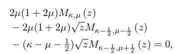
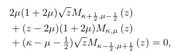
►From (13.14.2) and (13.14.3) has the same zeros as and has the same zeros as , hence the results given in §13.9 can be adopted.
►Asymptotic approximations to the zeros when the parameters and/or are large can be found by reversion of the uniform approximations provided in §§13.20 and 13.21.
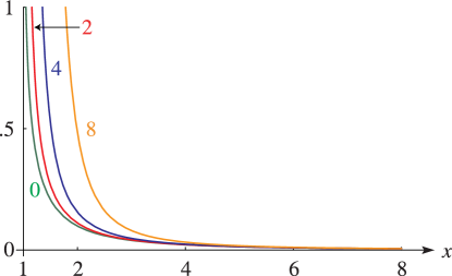
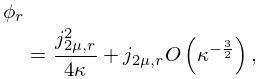
For example, if is fixed and is large, then the th positive zero of is given by
►
 ►
►
 ►
►
 ►
►
 ►
►
 ►
►
