日本金泽医科大学文凭毕业证哪里有卖【仿证 微kaa77788】】LeQ

SearchAdvancedHelp

(0.002 seconds)

11—20 of 316 matching pages

11: 30.17 Tables

… ►

Stratton et al. (1956) tabulates quantities closely related to ${\lambda }_n^m\left({\gamma }^2\right)$ and $a_{n,k}^m({\gamma }^2)$ for $0\le m\le 8$, $m\le n\le 8$, $-64\le {\gamma }^2\le 64$. Precision is 7S.

… ►

Hanish et al. (1970) gives ${\lambda }_n^m\left({\gamma }^2\right)$ and $S_n^{m(j)}(z,\gamma )$, $j=1,2$, and their first derivatives, for $0\le m\le 2$, $m\le n\le m+49$, $-1600\le {\gamma }^2\le 1600$. The range of $z$ is given by $1\le z\le 10$ if ${\gamma }^2>0$, or $z=-\mathrm{i}\xi$, $0\le \xi \le 2$ if . Precision is 18S.

►

EraŠevskaja et al. (1973, 1976) gives $S^{m(j)}(\mathrm{i}y,-\mathrm{i}c)$, $S^{m(j)}(z,\gamma )$ and their first derivatives for $j=1,2$, $0.5\le c\le 8$, $y=0,0.5,1,1.5$, $0.5\le \gamma \le 8$, $z=1.01,1.1,1.4,1.8$. Precision is 15S.

►

Van Buren et al. (1975) gives ${\lambda }_n^0\left({\gamma }^2\right)$, ${\mathrm{𝖯𝗌}}_n^0(x,{\gamma }^2)$ for $0\le n\le 49$, $-1600\le {\gamma }^2\le 1600$, $-1\le x\le 1$. Precision is 8S.

…

12: 33.25 Approximations

… ►Cody and Hillstrom (1970) provides rational approximations of the phase shift ${\sigma }_0\left(\eta \right)=\mathrm{ph}\mathrm{\Gamma }\left(1+\mathrm{i}\eta \right)$ (see (33.2.10)) for the ranges $0\le \eta \le 2$, $2\le \eta \le 4$, and $4\le \eta \le \mathrm{\infty }$. …

13: 12.3 Graphics

… ►

►►

Figure 12.3.5: $U(-8,x)$, $\overline{U}(-8,x)$, $F(-8,x)$, $-4\sqrt{2}\le x\le 4\sqrt{2}$. Magnify

… ►

►

►

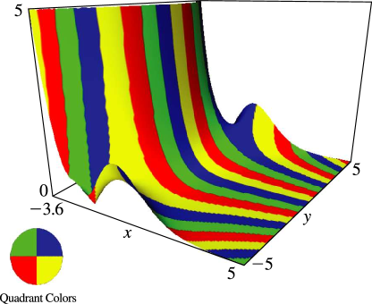
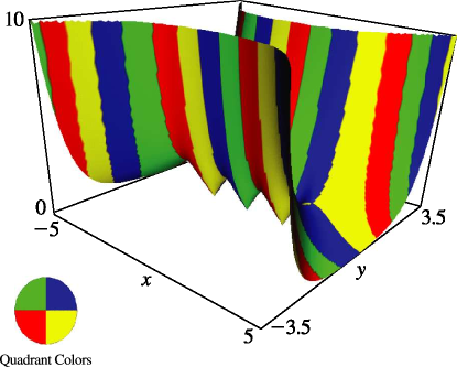
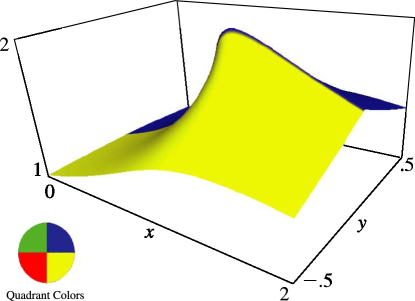
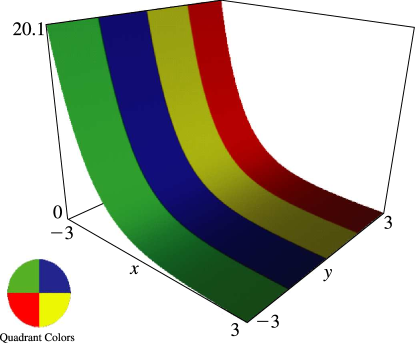
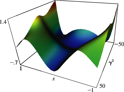
Figure 12.3.7: $U(a,x)$, $-2.5\le a\le 2.5$, $-2.5\le x\le 2.5$. Magnify 3D Help

►

►

►

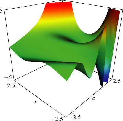
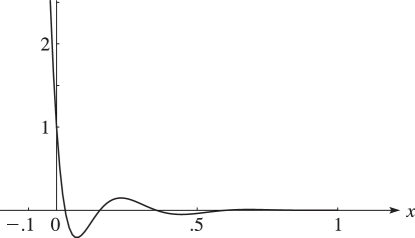
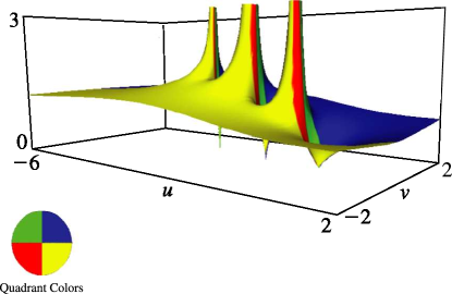
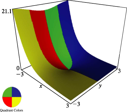
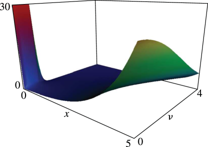
Figure 12.3.8: $V(a,x)$, $-2.5\le a\le 2.5$, $-2.5\le x\le 2.5$. Magnify 3D Help

… ►

►

►

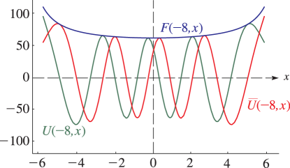
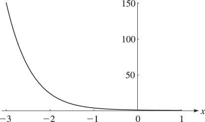
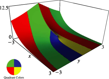
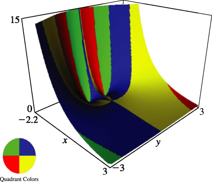
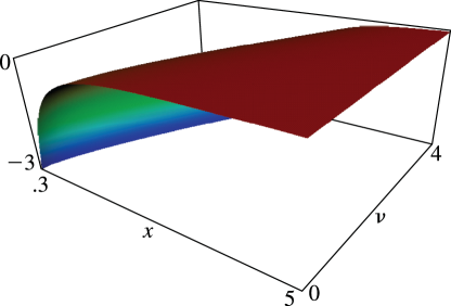
Figure 12.3.9: $U(3.5,x+\mathrm{i}y)$, $-3.6\le x\le 5$, $-5\le y\le 5$. Magnify 3D Help

►

►

►

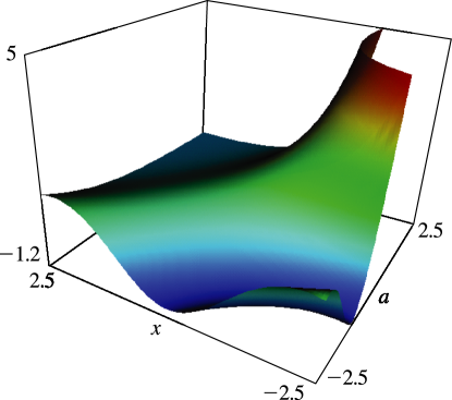
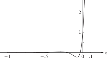
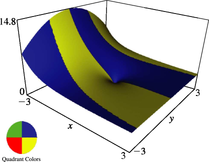
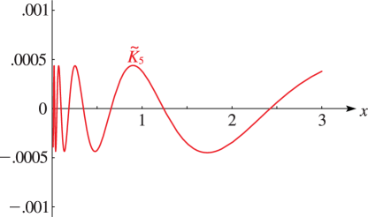
Figure 12.3.10: $U(-3.5,x+\mathrm{i}y)$, $-5\le x\le 5$, $-3.5\le y\le 3.5$. Magnify 3D Help

14: 15.3 Graphics

… ►

►►

Figure 15.3.2: $F(5,-10;1;x),-0.023\le x\le 1$. Magnify

►

►►

Figure 15.3.3: $F(1,-10;10;x),-3\le x\le 1$. Magnify

►

►►

Figure 15.3.4: $F(5,10;1;x),-1\le x\le 0.022$. Magnify

… ►

►

►

Figure 15.3.5: $F(\frac{4}{3},\frac{9}{16};\frac{14}{5};x+\mathrm{i}y),0\le x\le 2,-0.5\le y\le 0.5$. … Magnify 3D Help

►

►

►

Figure 15.3.6: $F(-3,\frac{3}{5};u+\mathrm{i}v;\frac{1}{2}),-6\le u\le 2,-2\le v\le 2$. … Magnify 3D Help

…

15: 8.3 Graphics

… ►

►

►

Figure 8.3.8: $\mathrm{\Gamma }(0.25,x+\mathrm{i}y)$, $-3\le x\le 3$, $-3\le y\le 3$. … Magnify 3D Help

►

►

►

Figure 8.3.9: $\gamma (0.25,x+\mathrm{i}y)$, $-3\le x\le 3$, $-3\le y\le 3$. … Magnify 3D Help

… ►

►

►

Figure 8.3.11: $\mathrm{\Gamma }(1,x+\mathrm{i}y)$, $-3\le x\le 3$, $-3\le y\le 3$. Magnify 3D Help

►

►

►

Figure 8.3.12: $\gamma (1,x+\mathrm{i}y)$, $-3\le x\le 3$, $-3\le y\le 3$. Magnify 3D Help

… ►

►

►

Figure 8.3.14: $\mathrm{\Gamma }(2.5,x+\mathrm{i}y)$, $-2.2\le x\le 3$, $-3\le y\le 3$. … Magnify 3D Help

…

16: 6.3 Graphics

… ►

►►

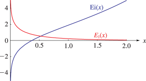
Figure 6.3.1: The exponential integrals $E_1\left(x\right)$ and $\mathrm{Ei}\left(x\right)$, . Magnify

►

►►

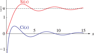
Figure 6.3.2: The sine and cosine integrals $\mathrm{Si}\left(x\right),\mathrm{Ci}\left(x\right)$, $0\le x\le 15$. Magnify

… ►

►

►

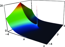
Figure 6.3.3: $|E_1\left(x+\mathrm{i}y\right)|$, $-4\le x\le 4$, $-4\le y\le 4$. … Magnify 3D Help

17: 10.26 Graphics

… ►

►

►

Figure 10.26.3: $I_{\nu }\left(x\right)$, $0\le x\le 5$, $0\le \nu \le 4$. Magnify 3D Help

►

►

►

Figure 10.26.4: $K_{\nu }\left(x\right)$, $0.1\le x\le 5$, $0\le \nu \le 4$. Magnify 3D Help

►

►

►

Figure 10.26.5: $I_{\nu }^{\prime }\left(x\right)$, $0\le x\le 5$, $0\le \nu \le 4$. Magnify 3D Help

►

►

►

Figure 10.26.6: $K_{\nu }^{\prime }\left(x\right)$, $0.3\le x\le 5$, $0\le \nu \le 4$. Magnify 3D Help

… ►

►►

Figure 10.26.10: ${\tilde{K}}_5\left(x\right)$, $0.01\le x\le 3$. Magnify

18: 30.7 Graphics

… ►

►

►

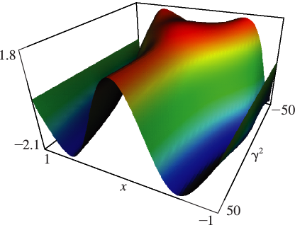
Figure 30.7.9: ${\mathrm{𝖯𝗌}}_2^0(x,{\gamma }^2)$, $-1\le x\le 1$, $-50\le {\gamma }^2\le 50$. Magnify 3D Help

►

►

►

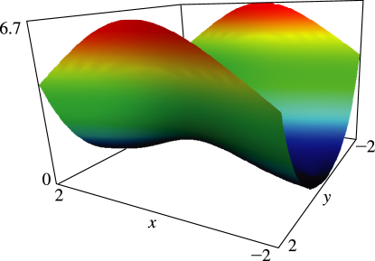
Figure 30.7.10: ${\mathrm{𝖯𝗌}}_3^1(x,{\gamma }^2)$, $-1\le x\le 1$, $-50\le {\gamma }^2\le 50$. Magnify 3D Help

… ►

►

►

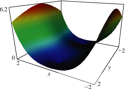
Figure 30.7.16: $|{\mathrm{𝑃𝑠}}_0^0(x+\mathrm{i}y,4)|$, $-2\le x\le 2$, $-2\le y\le 2$. Magnify 3D Help

►

►

►

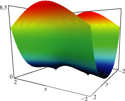
Figure 30.7.17: $|{\mathrm{𝑃𝑠}}_0^0(x+\mathrm{i}y,-4)|$, $-2\le x\le 2$, $-2\le y\le 2$. Magnify 3D Help

►

►

►

Figure 30.7.18: $|{\mathrm{𝑃𝑠}}_1^1(x+\mathrm{i}y,4)|$, $-2\le x\le 2$, $-2\le y\le 2$. Magnify 3D Help

…

19: 5.23 Approximations

… ►Cody and Hillstrom (1967) gives minimax rational approximations for $\ln \mathrm{\Gamma }\left(x\right)$ for the ranges $0.5\le x\le 1.5$, $1.5\le x\le 4$, $4\le x\le 12$; precision is variable. Hart et al. (1968) gives minimax polynomial and rational approximations to $\mathrm{\Gamma }\left(x\right)$ and $\ln \mathrm{\Gamma }\left(x\right)$ in the intervals $0\le x\le 1$, $8\le x\le 1000$, $12\le x\le 1000$; precision is variable. Cody et al. (1973) gives minimax rational approximations for $\psi \left(x\right)$ for the ranges $0.5\le x\le 3$ and ; precision is variable. … ►Luke (1969b) gives the coefficients to 20D for the Chebyshev-series expansions of $\mathrm{\Gamma }\left(1+x\right)$, $1/\mathrm{\Gamma }\left(1+x\right)$, $\mathrm{\Gamma }\left(x+3\right)$, $\ln \mathrm{\Gamma }\left(x+3\right)$, $\psi \left(x+3\right)$, and the first six derivatives of $\psi \left(x+3\right)$ for $0\le x\le 1$. …Clenshaw (1962) also gives 20D Chebyshev-series coefficients for $\mathrm{\Gamma }\left(1+x\right)$ and its reciprocal for $0\le x\le 1$. …

20: 35.11 Tables

… ►Tables of zonal polynomials are given in James (1964) for $|\kappa |\le 6$, Parkhurst and James (1974) for $|\kappa |\le 12$, and Muirhead (1982, p. 238) for $|\kappa |\le 5$. …