北海道教育大学证书【假证加微aptao168】1tSIPmf

SearchAdvancedHelp

(0.002 seconds)

21—30 of 821 matching pages

21: 22.5 Special Values

… ►For example, at $z=K+\mathrm{i}{K}^{\prime }$, $\mathrm{sn}(z,k)=1/k$, $d\mathrm{sn}(z,k)/dz=0$. … ►For example, $\mathrm{sn}(\frac{1}{2}K,k)={(1+k^{\prime })}^{-1/2}$. … ►

§22.5(ii) Limiting Values of $k$

… ►Expansions for $K,K^{\prime }$ as $k\to 0$ or $1$ are given in §§19.5, 19.12. … ►

22: 26.2 Basic Definitions

… ►Thus $231$ is the permutation $\sigma (1)=2$, $\sigma (2)=3$, $\sigma (3)=1$. … ►As an example, $\{1,1,1,2,4,4\}$ is a partition of 13. …See Table 26.2.1 for $n=0(1)50$. For the actual partitions ($\pi$) for $n=1(1)5$ see Table 26.4.1. … ►The example $\{1,1,1,2,4,4\}$ has six parts, three of which equal 1. …

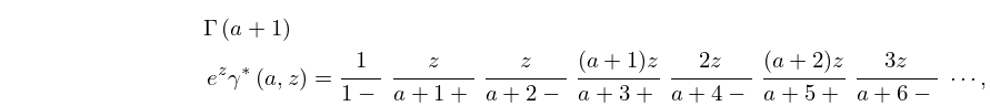
23: 8.9 Continued Fractions

… ►

8.9.1 $$\mathrm{\Gamma }\left(a+1\right){\mathrm{e}}^z{\gamma }^{\ast }(a,z)=\frac{1}{1-}\frac{z}{a+1+}\frac{z}{a+2-}\frac{(a+1)z}{a+3+}\frac{2z}{a+4-}\frac{(a+2)z}{a+5+}\frac{3z}{a+6-}\mathrm{\cdots },$$ $a\ne -1,-2,\mathrm{\dots }$,

ⓘ

Symbols:

$\mathrm{\Gamma }\left(z\right)$: gamma function, $\mathrm{e}$: base of natural logarithm, ${\gamma }^{\ast }(a,z)$: incomplete gamma function, $z$: complex variable and $a$: parameter

A&S Ref:

6.5.31 (in modified form.)

Permalink:

http://dlmf.nist.gov/8.9.E1

Encodings:

pMML, png, TeX

See also:

Annotations for §8.9 and Ch.8

►

8.9.2 $$z^{-a}{\mathrm{e}}^z\mathrm{\Gamma }(a,z)=\frac{z^{-1}}{1+}\frac{(1-a)z^{-1}}{1+}\frac{z^{-1}}{1+}\frac{(2-a)z^{-1}}{1+}\frac{2z^{-1}}{1+}\frac{(3-a)z^{-1}}{1+}\frac{3z^{-1}}{1+}\mathrm{\cdots },$$ .

ⓘ

Symbols:

$\pi$: the ratio of the circumference of a circle to its diameter, $\mathrm{e}$: base of natural logarithm, $\mathrm{\Gamma }(a,z)$: incomplete gamma function, $\mathrm{ph}$: phase, $z$: complex variable and $a$: parameter

Referenced by:

§8.19(vii)

Permalink:

http://dlmf.nist.gov/8.9.E2

Encodings:

pMML, png, TeX

See also:

Annotations for §8.9 and Ch.8

…

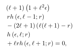
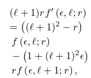
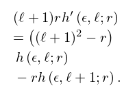
24: 33.17 Recurrence Relations and Derivatives

… ►

33.17.1 $$(\mathrm{\ell }+1)rf(ϵ,\mathrm{\ell }-1;r)-(2\mathrm{\ell }+1)\left(\mathrm{\ell }(\mathrm{\ell }+1)-r\right)f(ϵ,\mathrm{\ell };r)+\mathrm{\ell }\left(1+{(\mathrm{\ell }+1)}^2ϵ\right)rf(ϵ,\mathrm{\ell }+1;r)=0,$$

ⓘ

Symbols:

$f(ϵ,\mathrm{\ell };r)$: regular Coulomb function, $\mathrm{\ell }$: nonnegative integer, $r$: real variable and $ϵ$: real parameter

Permalink:

http://dlmf.nist.gov/33.17.E1

Encodings:

pMML, png, TeX

See also:

Annotations for §33.17 and Ch.33

►

33.17.2 $$(\mathrm{\ell }+1)\left(1+{\mathrm{\ell }}^2ϵ\right)rh(ϵ,\mathrm{\ell }-1;r)-(2\mathrm{\ell }+1)\left(\mathrm{\ell }(\mathrm{\ell }+1)-r\right)h(ϵ,\mathrm{\ell };r)+\mathrm{\ell }rh(ϵ,\mathrm{\ell }+1;r)=0,$$

ⓘ

Symbols:

$h(ϵ,\mathrm{\ell };r)$: irregular Coulomb function, $\mathrm{\ell }$: nonnegative integer, $r$: real variable and $ϵ$: real parameter

Permalink:

http://dlmf.nist.gov/33.17.E2

Encodings:

pMML, png, TeX

See also:

Annotations for §33.17 and Ch.33

►

33.17.3 $$(\mathrm{\ell }+1)r{f}^{\prime }(ϵ,\mathrm{\ell };r)=\left({(\mathrm{\ell }+1)}^2-r\right)f(ϵ,\mathrm{\ell };r)-\left(1+{(\mathrm{\ell }+1)}^2ϵ\right)rf(ϵ,\mathrm{\ell }+1;r),$$

ⓘ

Symbols:

$f(ϵ,\mathrm{\ell };r)$: regular Coulomb function, $\mathrm{\ell }$: nonnegative integer, $r$: real variable and $ϵ$: real parameter

Permalink:

http://dlmf.nist.gov/33.17.E3

Encodings:

pMML, png, TeX

See also:

Annotations for §33.17 and Ch.33

►

33.17.4 $$(\mathrm{\ell }+1)r{h}^{\prime }(ϵ,\mathrm{\ell };r)=\left({(\mathrm{\ell }+1)}^2-r\right)h(ϵ,\mathrm{\ell };r)-rh(ϵ,\mathrm{\ell }+1;r).$$

ⓘ

Symbols:

$h(ϵ,\mathrm{\ell };r)$: irregular Coulomb function, $\mathrm{\ell }$: nonnegative integer, $r$: real variable and $ϵ$: real parameter

Permalink:

http://dlmf.nist.gov/33.17.E4

Encodings:

pMML, png, TeX

See also:

Annotations for §33.17 and Ch.33

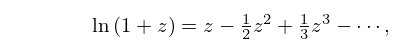
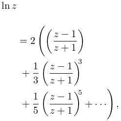
25: 4.6 Power Series

… ►

4.6.1 $$\ln \left(1+z\right)=z-\frac{1}{2}{z}^2+\frac{1}{3}{z}^3-\mathrm{\cdots },$$ $|z|\le 1$, $z\ne -1$,

ⓘ

Symbols:

$\ln z$: principal branch of logarithm function and $z$: complex variable

A&S Ref:

4.1.24

Referenced by:

§4.45(i), §4.6(i), (8.15.2)

Permalink:

http://dlmf.nist.gov/4.6.E1

Encodings:

pMML, png, TeX

See also:

Annotations for §4.6(i), §4.6 and Ch.4

… ►

4.6.3 $$\ln z=(z-1)-\frac{1}{2}{(z-1)}^2+\frac{1}{3}{(z-1)}^3-\mathrm{\cdots },$$ $|z-1|\le 1$, $z\ne 0$,

ⓘ

Symbols:

$\ln z$: principal branch of logarithm function and $z$: complex variable

A&S Ref:

4.1.26

Permalink:

http://dlmf.nist.gov/4.6.E3

Encodings:

pMML, png, TeX

See also:

Annotations for §4.6(i), §4.6 and Ch.4

►

4.6.4 $$\ln z=2\left(\left(\frac{z-1}{z+1}\right)+\frac{1}{3}{\left(\frac{z-1}{z+1}\right)}^3+\frac{1}{5}{\left(\frac{z-1}{z+1}\right)}^5+\mathrm{\cdots }\right),$$ $\mathrm{\Re }z\ge 0$, $z\ne 0$,

ⓘ

Symbols:

$\ln z$: principal branch of logarithm function, $\mathrm{\Re }$: real part and $z$: complex variable

A&S Ref:

4.1.27

Permalink:

http://dlmf.nist.gov/4.6.E4

Encodings:

pMML, png, TeX

See also:

Annotations for §4.6(i), §4.6 and Ch.4

… ►valid when $a$ is any real or complex constant and . If $a=0,1,2,\mathrm{\dots }$, then the series terminates and $z$ is unrestricted. …

26: 14.33 Tables

… ►

Abramowitz and Stegun (1964, Chapter 8) tabulates ${𝖯}_n\left(x\right)$ for $n=0(1)3,9,10$, $x=0(.01)1$, 5–8D; ${𝖯}_n^{\prime }\left(x\right)$ for $n=1(1)4,9,10$, $x=0(.01)1$, 5–7D; ${𝖰}_n\left(x\right)$ and ${𝖰}_n^{\prime }\left(x\right)$ for $n=0(1)3,9,10$, $x=0(.01)1$, 6–8D; $P_n\left(x\right)$ and $P_n^{\prime }\left(x\right)$ for $n=0(1)5,9,10$, $x=1(.2)10$, 6S; $Q_n\left(x\right)$ and $Q_n^{\prime }\left(x\right)$ for $n=0(1)3,9,10$, $x=1(.2)10$, 6S. (Here primes denote derivatives with respect to $x$.)

►

Zhang and Jin (1996, Chapter 4) tabulates ${𝖯}_n\left(x\right)$ for $n=2(1)5,10$, $x=0(.1)1$, 7D; ${𝖯}_n\left(\cos \theta \right)$ for $n=1(1)4,10$, $\theta =0(5^{\circ }){90}^{\circ }$, 8D; ${𝖰}_n\left(x\right)$ for $n=0(1)2,10$, $x=0(.1)0.9$, 8S; ${𝖰}_n\left(\cos \theta \right)$ for $n=0(1)3,10$, $\theta =0(5^{\circ }){90}^{\circ }$, 8D; ${𝖯}_n^m\left(x\right)$ for $m=1(1)4$, $n-m=0(1)2$, $n=10$, $x=0,0.5$, 8S; ${𝖰}_n^m\left(x\right)$ for $m=1(1)4$, $n=0(1)2,10$, 8S; ${𝖯}_{\nu }^m\left(\cos \theta \right)$ for $m=0(1)3$, $\nu =0(.25)5$, $\theta =0({15}^{\circ }){90}^{\circ }$, 5D; $P_n\left(x\right)$ for $n=2(1)5,10$, $x=1(1)10$, 7S; $Q_n\left(x\right)$ for $n=0(1)2,10$, $x=2(1)10$, 8S. Corresponding values of the derivative of each function are also included, as are 6D values of the first 5 $\nu$-zeros of ${𝖯}_{\nu }^m\left(\cos \theta \right)$ and of its derivative for $m=0(1)4$, $\theta ={10}^{\circ },{30}^{\circ },{150}^{\circ }$.

►

Belousov (1962) tabulates ${𝖯}_n^m\left(\cos \theta \right)$ (normalized) for $m=0(1)36$, $n-m=0(1)56$, $\theta =0({2.5}^{\circ }){90}^{\circ }$, 6D.

►

Žurina and Karmazina (1964, 1965) tabulate the conical functions ${𝖯}_{-\frac{1}{2}+\mathrm{i}\tau }\left(x\right)$ for $\tau =0(.01)50$, $x=-0.9(.1)0.9$, 7S; $P_{-\frac{1}{2}+\mathrm{i}\tau }\left(x\right)$ for $\tau =0(.01)50$, $x=1.1(.1)2(.2)5(.5)10(10)60$, 7D. Auxiliary tables are included to facilitate computation for larger values of $\tau$ when .

►

Žurina and Karmazina (1963) tabulates the conical functions ${𝖯}_{-\frac{1}{2}+\mathrm{i}\tau }^1\left(x\right)$ for $\tau =0(.01)25$, $x=-0.9(.1)0.9$, 7S; $P_{-\frac{1}{2}+\mathrm{i}\tau }^1\left(x\right)$ for $\tau =0(.01)25$, $x=1.1(.1)2(.2)5(.5)10(10)60$, 7S. Auxiliary tables are included to assist computation for larger values of $\tau$ when .

…

27: 29.21 Tables

… ►

Ince (1940a) tabulates the eigenvalues $a_{\nu }^m\left(k^2\right)$, $b_{\nu }^{m+1}\left(k^2\right)$ (with $a_{\nu }^{2m+1}$ and $b_{\nu }^{2m+1}$ interchanged) for $k^2=0.1,0.5,0.9$, $\nu =-\frac{1}{2},0(1)25$, and $m=0,1,2,3$. Precision is 4D.

►

Arscott and Khabaza (1962) tabulates the coefficients of the polynomials $P$ in Table 29.12.1 (normalized so that the numerically largest coefficient is unity, i.e. monic polynomials), and the corresponding eigenvalues $h$ for $k^2=0.1(.1)0.9$, $n=1(1)30$. Equations from §29.6 can be used to transform to the normalization adopted in this chapter. Precision is 6S.

28: 16.12 Products

… ►

16.12.1 $${}_0{}^{}F_1^{}(-;a;z){}_0{}^{}F_1^{}(-;b;z)={}_2{}^{}F_3^{}(\genfrac{}{}{0pt}{}{\frac{1}{2}(a+b),\frac{1}{2}(a+b-1)}{a,b,a+b-1};4z).$$

ⓘ

Symbols:

${}_p{}^{}F_q^{}(a_1,\mathrm{\dots },a_p;b_1,\mathrm{\dots },b_q;z)$ or ${}_p{}^{}F_q^{}(\genfrac{}{}{0pt}{}{a_1,\mathrm{\dots },a_p}{b_1,\mathrm{\dots },b_q};z)$: alternatively ${}_p{}^{}F_q^{}(𝐚;𝐛;z)$ or ${}_p{}^{}F_q^{}(\genfrac{}{}{0pt}{}{𝐚}{𝐛};z)$
generalized hypergeometric function, $z$: complex variable, $a,a_1,\mathrm{\dots },a_p$: real or complex parameters and $b,b_1,\mathrm{\dots },b_q$: real or complex parameters

Referenced by:

(10.8.3), §10.8, §10.8, §16.12, Erratum (V1.0.17) for Section 10.8

Permalink:

http://dlmf.nist.gov/16.12.E1

Encodings:

pMML, png, TeX

See also:

Annotations for §16.12 and Ch.16

… ►

16.12.2 $${\left({}_2{}^{}F_1^{}(\genfrac{}{}{0pt}{}{a,b}{a+b+\frac{1}{2}};z)\right)}^2={}_3{}^{}F_2^{}(\genfrac{}{}{0pt}{}{2a,2b,a+b}{a+b+\frac{1}{2},2a+2b};z).$$

ⓘ

Symbols:

${}_2{}^{}F_1^{}(a,b;c;z)$: $=F(a,b;c;z)$ notation for Gauss’ hypergeometric function, ${}_p{}^{}F_q^{}(a_1,\mathrm{\dots },a_p;b_1,\mathrm{\dots },b_q;z)$ or ${}_p{}^{}F_q^{}(\genfrac{}{}{0pt}{}{a_1,\mathrm{\dots },a_p}{b_1,\mathrm{\dots },b_q};z)$: alternatively ${}_p{}^{}F_q^{}(𝐚;𝐛;z)$ or ${}_p{}^{}F_q^{}(\genfrac{}{}{0pt}{}{𝐚}{𝐛};z)$
generalized hypergeometric function, $z$: complex variable, $a,a_1,\mathrm{\dots },a_p$: real or complex parameters and $b,b_1,\mathrm{\dots },b_q$: real or complex parameters

Referenced by:

§16.12, §17.9(iii), Erratum (V1.1.12) for Subsection 17.9(iii)

Permalink:

http://dlmf.nist.gov/16.12.E2

Encodings:

pMML, png, TeX

See also:

Annotations for §16.12 and Ch.16

… ►

16.12.3 $${\left({}_2{}^{}F_1^{}(\genfrac{}{}{0pt}{}{a,b}{c};z)\right)}^2=\sum _{k=0}^{\mathrm{\infty }}\frac{{\left(2a\right)}_k{\left(2b\right)}_k{\left(c-\frac{1}{2}\right)}_k}{{\left(c\right)}_k{\left(2c-1\right)}_{k}k!}{}_4{}^{}F_3^{}(\genfrac{}{}{0pt}{}{-\frac{1}{2}k,\frac{1}{2}(1-k),a+b-c+\frac{1}{2},\frac{1}{2}}{a+\frac{1}{2},b+\frac{1}{2},\frac{3}{2}-k-c};1)z^k,$$ .

ⓘ

Symbols:

${}_2{}^{}F_1^{}(a,b;c;z)$: $=F(a,b;c;z)$ notation for Gauss’ hypergeometric function, ${}_p{}^{}F_q^{}(a_1,\mathrm{\dots },a_p;b_1,\mathrm{\dots },b_q;z)$ or ${}_p{}^{}F_q^{}(\genfrac{}{}{0pt}{}{a_1,\mathrm{\dots },a_p}{b_1,\mathrm{\dots },b_q};z)$: alternatively ${}_p{}^{}F_q^{}(𝐚;𝐛;z)$ or ${}_p{}^{}F_q^{}(\genfrac{}{}{0pt}{}{𝐚}{𝐛};z)$
generalized hypergeometric function, ${\left(a\right)}_n$: Pochhammer’s symbol (or shifted factorial), $!$: factorial (as in $n!$), $z$: complex variable, $a,a_1,\mathrm{\dots },a_p$: real or complex parameters and $b,b_1,\mathrm{\dots },b_q$: real or complex parameters

Referenced by:

§16.12

Permalink:

http://dlmf.nist.gov/16.12.E3

Encodings:

pMML, png, TeX

See also:

Annotations for §16.12 and Ch.16

…

29: 26.12 Plane Partitions

… ►An equivalent definition is that a plane partition is a finite subset of $\mathbb{N}\times \mathbb{N}\times \mathbb{N}$ with the property that if $(r,s,t)\in \pi$ and $(1,1,1)\le (h,j,k)\le (r,s,t)$, then $(h,j,k)$ must be an element of $\pi$. … ►The complement of $\pi \subseteq B(r,s,t)$ is ${\pi }^c=\{(h,j,k)|(r-h+1,s-j+1,t-k+1)\notin \pi \}$. …in $B(2r+1,2s,2t)$ it is …in $B(2r+1,2s+1,2t)$ it is … ►in $B(2r+1,2r+1,2t)$ it is …

30: 18.8 Differential Equations

… ►

Table 18.8.1: Classical OP’s: differential equations $A(x)f^{\prime \prime }(x)+B(x)f^{\prime }(x)+C(x)f(x)+{\lambda }_{n}f(x)=0$.

► ►►►►►►

#	$f(x)$	$A(x)$	$B(x)$	$C(x)$	${\lambda }_n$
…
7	$P_n\left(x\right)$	$1-x^2$	$-2x$	$0$	$n(n+1)$
…
10	${\mathrm{e}}^{-\frac{1}{2}x}{x}^{\frac{1}{2}\alpha }{L}_n^{(\alpha )}\left(x\right)$	$x$	$1$	$-\frac{1}{4}x-\frac{1}{4}{\alpha }^2{x}^{-1}$	$n+\frac{1}{2}(\alpha +1)$
11	${\mathrm{e}}^{-n^{-1}x}{x}^{\mathrm{\ell }+1}{L}_{n-\mathrm{\ell }-1}^{(2\mathrm{\ell }+1)}\left(2n^{-1}x\right)$	$1$	$0$	$\frac{2}{x}-\frac{\mathrm{\ell }(\mathrm{\ell }+1)}{x^2}$	$-\frac{1}{n^2}$
12	$H_n\left(x\right)$	$1$	$-2x$	$0$	$2n$
…

►

►Item 11 of Table 18.8.1 yields (18.39.36) for $Z=1$.