办假的科罗拉多学院文凭毕业证【somewhat微aptao168】bigrf

SearchAdvancedHelp

(0.002 seconds)

11—20 of 28 matching pages

11: 19.33 Triaxial Ellipsoids

… ►

19.33.5 $$V(\lambda )=Q{R}_F(a^2+\lambda ,b^2+\lambda ,c^2+\lambda ),$$

ⓘ

Symbols:

$R_F(x,y,z)$: symmetric elliptic integral of first kind, $Q$: charge and $V(\lambda )$: potential

Permalink:

http://dlmf.nist.gov/19.33.E5

Encodings:

pMML, png, TeX

See also:

Annotations for §19.33(ii), §19.33 and Ch.19

… ►

19.33.6 $$1/C=R_F(a^2,b^2,c^2).$$

ⓘ

Symbols:

$R_F(x,y,z)$: symmetric elliptic integral of first kind and $C$: electric capacity

Permalink:

http://dlmf.nist.gov/19.33.E6

Encodings:

pMML, png, TeX

See also:

Annotations for §19.33(ii), §19.33 and Ch.19

… ►

19.33.11 $$U=\frac{1}{2}{(\alpha \beta \gamma )}^2{R}_F({\alpha }^2,{\beta }^2,{\gamma }^2){\int }_0^{\mathrm{\infty }}{(g(r))}^{2}dr,$$

ⓘ

Symbols:

$R_F(x,y,z)$: symmetric elliptic integral of first kind, $dx$: differential of $x$ , $\int$: integral, $\alpha$: positive constant, $\beta$: positive constant, $\gamma$: positive constant, $U$: energy and $g(r)$: function

Permalink:

http://dlmf.nist.gov/19.33.E11

Encodings:

pMML, png, TeX

See also:

Annotations for §19.33(iv), §19.33 and Ch.19

…

12: 19.27 Asymptotic Approximations and Expansions

… ►

§19.27(ii) $R_F(x,y,z)$

… ►

19.27.2 $$R_F(x,y,z)=\frac{1}{2\sqrt{z}}\left(\ln \frac{8z}{a+g}\right)\left(1+O\left(\frac{a}{z}\right)\right),$$ $a/z\to 0$.

ⓘ

Symbols:

$O\left(x\right)$: order not exceeding, $R_F(x,y,z)$: symmetric elliptic integral of first kind, $\ln z$: principal branch of logarithm function, $a$ and $g$

Referenced by:

§19.20(iii), §19.27(ii)

Permalink:

http://dlmf.nist.gov/19.27.E2

Encodings:

pMML, png, TeX

See also:

Annotations for §19.27(ii), §19.27 and Ch.19

►

19.27.3 $$R_F(x,y,z)=R_F(0,y,z)-\frac{1}{\sqrt{h}}\left(\sqrt{\frac{x}{h}}+O\left(\frac{x}{h}\right)\right),$$ $x/h\to 0$.

ⓘ

Symbols:

$O\left(x\right)$: order not exceeding, $R_F(x,y,z)$: symmetric elliptic integral of first kind and $h$

Permalink:

http://dlmf.nist.gov/19.27.E3

Encodings:

pMML, png, TeX

See also:

Annotations for §19.27(ii), §19.27 and Ch.19

… ►

19.27.11 $$R_J(x,y,z,p)=\frac{3}{p}{R}_F(x,y,z)-\frac{3\pi }{2p^{3/2}}\left(1+O\left(\sqrt{\frac{c}{p}}\right)\right),$$ $c/p\to 0$.

ⓘ

Symbols:

$O\left(x\right)$: order not exceeding, $R_F(x,y,z)$: symmetric elliptic integral of first kind, $R_J(x,y,z,p)$: symmetric elliptic integral of third kind, $\pi$: the ratio of the circumference of a circle to its diameter and $c$

Referenced by:

§19.20(iii)

Permalink:

http://dlmf.nist.gov/19.27.E11

Encodings:

pMML, png, TeX

See also:

Annotations for §19.27(v), §19.27 and Ch.19

…

13: 19.34 Mutual Inductance of Coaxial Circles

… ►

19.34.5 $$\frac{3c^2}{8\pi ab}M=3R_F(0,r_{+}^2,r_{-}^2)-2r_{-}^2{R}_D(0,r_{+}^2,r_{-}^2),$$

ⓘ

Symbols:

$R_D(x,y,z)$: elliptic integral symmetric in only two variables, $R_F(x,y,z)$: symmetric elliptic integral of first kind, $\pi$: the ratio of the circumference of a circle to its diameter, $M$: mutual inductance and $r_{\pm }$

Permalink:

http://dlmf.nist.gov/19.34.E5

Encodings:

pMML, png, TeX

See also:

Annotations for §19.34 and Ch.19

… ►

19.34.6 $$\frac{c^2}{2\pi }M=(r_{+}^2+r_{-}^2)R_F(0,r_{+}^2,r_{-}^2)-4R_G(0,r_{+}^2,r_{-}^2).$$

ⓘ

Symbols:

$R_F(x,y,z)$: symmetric elliptic integral of first kind, $R_G(x,y,z)$: symmetric elliptic integral of second kind, $\pi$: the ratio of the circumference of a circle to its diameter, $M$: mutual inductance and $r_{\pm }$

Referenced by:

§19.34

Permalink:

http://dlmf.nist.gov/19.34.E6

Encodings:

pMML, png, TeX

See also:

Annotations for §19.34 and Ch.19

…

14: 19.20 Special Cases

… ►

§19.20(i) $R_F(x,y,z)$

… ►

$$R_F(x,x,x)=x^{-1/2},$$

►

$$R_F(\lambda x,\lambda y,\lambda z)={\lambda }^{-1/2}{R}_F(x,y,z),$$

►

$$R_F(x,y,y)=R_C(x,y),$$

… ►

$$R_F(0,0,z)=\mathrm{\infty }.$$

…

15: 19.25 Relations to Other Functions

… ►

$K\left(k\right)=R_F(0,k_{}^{\prime }{}_{}{}^2,1),$

… ►

19.25.17 $$F(\varphi ,k)=R_F(x,y,z),$$

ⓘ

Symbols:

$R_F(x,y,z)$: symmetric elliptic integral of first kind, $F(\varphi ,k)$: Legendre’s incomplete elliptic integral of the first kind, $\varphi$: real or complex argument and $k$: real or complex modulus

Referenced by:

§19.15

Permalink:

http://dlmf.nist.gov/19.25.E17

Encodings:

pMML, png, TeX

See also:

Annotations for §19.25(i), §19.25 and Ch.19

… ►then the five nontrivial permutations of $x,y,z$ that leave $R_F$ invariant change $k^2$ ($=(z-y)/(z-x)$) into $1/k^2$, $k_{}^{\prime }{}_{}{}^2$, $1/k_{}^{\prime }{}_{}{}^2$, $-k^2/k_{}^{\prime }{}_{}{}^2$, $-k_{}^{\prime }{}_{}{}^2/k^2$, and $\sin \varphi$ ($=\sqrt{(z-x)/z}$) into $k\sin \varphi$, $-\mathrm{i}\tan \varphi$, $-\mathrm{i}{k}^{\prime }\tan \varphi$, $(k^{\prime }\sin \varphi )/\sqrt{1-k^2{\sin }^2\varphi }$, $-\mathrm{i}k\sin \varphi /\sqrt{1-k^2{\sin }^2\varphi }$. … ►

19.25.20 $$\mathrm{el1}(x,k_c)=R_F(r,r+k_c^2,r+1),$$

ⓘ

Symbols:

$\mathrm{el1}(x,k_c)$: Bulirsch’s incomplete elliptic integral of the first kind, $R_F(x,y,z)$: symmetric elliptic integral of first kind, $k$: real or complex modulus and $r$: inverse

Permalink:

http://dlmf.nist.gov/19.25.E20

Encodings:

pMML, png, TeX

See also:

Annotations for §19.25(ii), §19.25 and Ch.19

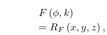
… ►Inversions of 12 elliptic integrals of the first kind, producing the 12 Jacobian elliptic functions, are combined and simplified by using the properties of $R_F(x,y,z)$. …

16: 19.23 Integral Representations

… ►

19.23.1 $$R_F(0,y,z)={\int }_0^{\pi /2}{(y{\cos }^2\theta +z{\sin }^2\theta )}^{-1/2}d\theta ,$$

ⓘ

Symbols:

$R_F(x,y,z)$: symmetric elliptic integral of first kind, $\pi$: the ratio of the circumference of a circle to its diameter, $\cos z$: cosine function, $dx$: differential of $x$ , $\int$: integral and $\sin z$: sine function

Referenced by:

§19.23, §19.23

Permalink:

http://dlmf.nist.gov/19.23.E1

Encodings:

pMML, png, TeX

See also:

Annotations for §19.23 and Ch.19

… ►

19.23.4 $$R_F(0,y,z)=\frac{2}{\pi }{\int }_0^{\pi /2}{R}_C(y,z{\cos }^2\theta )d\theta =\frac{2}{\pi }{\int }_0^{\mathrm{\infty }}{R}_C(y{\cosh }^{2}t,z)dt.$$

ⓘ

Symbols:

$R_C(x,y)$: Carlson’s combination of inverse circular and inverse hyperbolic functions, $R_F(x,y,z)$: symmetric elliptic integral of first kind, $\pi$: the ratio of the circumference of a circle to its diameter, $\cos z$: cosine function, $dx$: differential of $x$ , $\cosh z$: hyperbolic cosine function and $\int$: integral

Referenced by:

§19.23

Permalink:

http://dlmf.nist.gov/19.23.E4

Encodings:

pMML, png, TeX

See also:

Annotations for §19.23 and Ch.19

►

19.23.5 $$R_F(x,y,z)=\frac{2}{\pi }{\int }_0^{\pi /2}{R}_C(x,y{\cos }^2\theta +z{\sin }^2\theta )d\theta ,$$ $\mathrm{\Re }y>0$, $\mathrm{\Re }z>0$,

ⓘ

Symbols:

$R_C(x,y)$: Carlson’s combination of inverse circular and inverse hyperbolic functions, $R_F(x,y,z)$: symmetric elliptic integral of first kind, $\pi$: the ratio of the circumference of a circle to its diameter, $\cos z$: cosine function, $dx$: differential of $x$ , $\int$: integral, $\mathrm{\Re }$: real part and $\sin z$: sine function

Referenced by:

§19.2(iv), §19.23

Permalink:

http://dlmf.nist.gov/19.23.E5

Encodings:

pMML, png, TeX

See also:

Annotations for §19.23 and Ch.19

►

19.23.6 $$4\pi R_F(x,y,z)={\int }_0^{2\pi }{\int }_0^{\pi }\frac{\sin \theta d\theta d\varphi }{{(x{\sin }^2\theta {\cos }^2\varphi +y{\sin }^2\theta {\sin }^2\varphi +z{\cos }^2\theta )}^{1/2}},$$

ⓘ

Symbols:

$R_F(x,y,z)$: symmetric elliptic integral of first kind, $\pi$: the ratio of the circumference of a circle to its diameter, $\cos z$: cosine function, $dx$: differential of $x$ , $\int$: integral, $\sin z$: sine function and $\varphi$: real or complex argument

Referenced by:

§19.16(ii), §19.23

Permalink:

http://dlmf.nist.gov/19.23.E6

Encodings:

pMML, png, TeX

See also:

Annotations for §19.23 and Ch.19

…

17: 19.30 Lengths of Plane Curves

… ►

19.30.3 $$s/a=E(\varphi ,k)=R_F(c-1,c-k^2,c)-\frac{1}{3}{k}^2{R}_D(c-1,c-k^2,c),$$

ⓘ

Symbols:

$R_D(x,y,z)$: elliptic integral symmetric in only two variables, $R_F(x,y,z)$: symmetric elliptic integral of first kind, $E(\varphi ,k)$: Legendre’s incomplete elliptic integral of the second kind, $\varphi$: real or complex argument, $k$: real or complex modulus and $s$: arclength

Referenced by:

§19.30(i)

Permalink:

http://dlmf.nist.gov/19.30.E3

Encodings:

pMML, png, TeX

See also:

Annotations for §19.30(i), §19.30 and Ch.19

… ►

19.30.6 $$\frac{\partial s}{\partial (1/k)}=\sqrt{a^2-b^2}F(\varphi ,k)=\sqrt{a^2-b^2}{R}_F(c-1,c-k^2,c),$$ $k^2=(a^2-b^2)/(a^2+\lambda )$, $c={\csc }^2\varphi$.

ⓘ

Symbols:

$R_F(x,y,z)$: symmetric elliptic integral of first kind, $\csc z$: cosecant function, $F(\varphi ,k)$: Legendre’s incomplete elliptic integral of the first kind, $\frac{\partial f}{\partial x}$: partial derivative of $f$ with respect to $x$ , $\partial x$: partial differential of $x$ , $\varphi$: real or complex argument, $k$: real or complex modulus and $s$: arclength

Referenced by:

§19.30(i)

Permalink:

http://dlmf.nist.gov/19.30.E6

Encodings:

pMML, png, TeX

See also:

Annotations for §19.30(i), §19.30 and Ch.19

… ►

19.30.11 $$s=2a^2{\int }_0^r\frac{dt}{\sqrt{4a^4-t^4}}=\sqrt{2a^2}{R}_F(q-1,q,q+1),$$ $q=2a^2/r^2=\sec \left(2\theta \right)$,

ⓘ

Symbols:

$R_F(x,y,z)$: symmetric elliptic integral of first kind, $dx$: differential of $x$ , $\int$: integral, $\sec z$: secant function, $r$: length, $q$ and $s$: arclength

Permalink:

http://dlmf.nist.gov/19.30.E11

Encodings:

pMML, png, TeX

See also:

Annotations for §19.30(iii), §19.30 and Ch.19

… ►

19.30.13 $$P=4\sqrt{2a^2}{R}_F(0,1,2)=\sqrt{2a^2}\times \mathrm{5.24411\hspace{0.33em}51}\mathrm{\dots }=4aK\left(1/\sqrt{2}\right)=a\times \mathrm{7.41629\hspace{0.33em}87}\mathrm{\dots }.$$

ⓘ

Symbols:

$R_F(x,y,z)$: symmetric elliptic integral of first kind, $K\left(k\right)$: Legendre’s complete elliptic integral of the first kind and $P$: length

Notes:

For more digits see OEIS Sequence A064853; see also Sloane (2003).

Permalink:

http://dlmf.nist.gov/19.30.E13

Encodings:

pMML, png, TeX

See also:

Annotations for §19.30(iii), §19.30 and Ch.19

…

18: 19.31 Probability Distributions

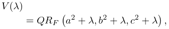
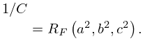
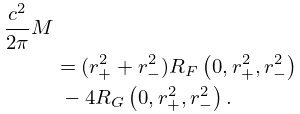
… ► $R_G(x,y,z)$ and $R_F(x,y,z)$ occur as the expectation values, relative to a normal probability distribution in ${ℝ}^2$ or ${ℝ}^3$, of the square root or reciprocal square root of a quadratic form. …§19.16(iii) shows that for $n=3$ the incomplete cases of $R_F$ and $R_G$ occur when $\mu =-1/2$ and $\mu =1/2$, respectively, while their complete cases occur when $n=2$. …

19: 19.15 Advantages of Symmetry

… ►Symmetry in $x,y,z$ of $R_F(x,y,z)$, $R_G(x,y,z)$, and $R_J(x,y,z,p)$ replaces the five transformations (19.7.2), (19.7.4)–(19.7.7) of Legendre’s integrals; compare (19.25.17). …

20: 19.17 Graphics

… ►For $R_F$, $R_G$, and $R_J$, which are symmetric in $x,y,z$, we may further assume that $z$ is the largest of $x,y,z$ if the variables are real, then choose $z=1$, and consider only $0\le x\le 1$ and $0\le y\le 1$. … ►To view $R_F(0,y,1)$ and $2R_G(0,y,1)$ for complex $y$, put $y=1-k^2$, use (19.25.1), and see Figures 19.3.7–19.3.12. ►

►►

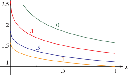
Figure 19.17.1: $R_F(x,y,1)$ for $0\le x\le 1$, $y=0,\mathrm{\hspace{0.17em}0.1},\mathrm{\hspace{0.17em}0.5},\mathrm{\hspace{0.17em}1}$. … Magnify

… ►To view $R_F(0,y,1)$ and $2R_G(0,y,1)$ for complex $y$, put $y=1-k^2$, use (19.25.1), and see Figures 19.3.7–19.3.12. …