%E5%8D%9A%E5%BD%A9%E6%8E%A8%E5%B9%BF%E8%AF%9D%E6%9C%AF,%E5%8D%9A%E5%BD%A9%E6%8E%A8%E5%B9%BF%E6%B8%A0%E9%81%93,%E5%8D%9A%E5%BD%A9%E5%BC%95%E6%B5%81%E6%96%B9%E5%BC%8F,%E3%80%90%E6%89%93%E5%BC%80%E7%BD%91%E5%9D%80%E2%88%B633kk88.com%E3%80%91%E5%8D%9A%E5%BD%A9%E6%8E%A8%E5%B9%BF%E6%8A%80%E5%B7%A7,%E5%8D%9A%E5%BD%A9seo%E6%8E%A8%E5%B9%BF%E6%B8%A0%E9%81%93,%E5%8D%9A%E5%BD%A9%E5%BC%95%E6%B5%81%E6%8A%80%E5%B7%A7,%E5%8D%9A%E5%BD%A9%E5%85%AC%E5%8F%B8%E6%8E%A8%E5%B9%BF%E6%96%B9%E6%B3%95,%E5%8D%9A%E5%BD%A9%E5%AE%A2%E6%88%B7%E8%AF%9D%E6%9C%AF,%E3%80%90%E5%8D%9A%E5%BD%A9%E5%9C%B0%E5%9D%80%E2%88%B633kk88.com%E3%80%91

SearchAdvancedHelp

(0.053 seconds)

11—20 of 603 matching pages

11: 30.3 Eigenvalues

… ►

30.3.11 $${\mathrm{\ell }}_8=2{(4m^2-1)}^{2}A+\frac{1}{16}B+\frac{1}{8}C+\frac{1}{2}D,$$

ⓘ

Symbols:

$m$: nonnegative integer, ${\mathrm{\ell }}_j$: coefficients, $A$ , $B$ , $C$ and $D$

Permalink:

http://dlmf.nist.gov/30.3.E11

Encodings:

pMML, png, TeX

See also:

Annotations for §30.3(iv), §30.3 and Ch.30

►

$$A=\frac{(n-m-1)(n-m)(n+m-1)(n+m)}{{(2n-5)}^2(2n-3){(2n-1)}^7(2n+1){(2n+3)}^2}-\frac{(n-m+1)(n-m+2)(n+m+1)(n+m+2)}{{(2n-1)}^2(2n+1){(2n+3)}^7(2n+5){(2n+7)}^2},$$

►

$$B=\frac{(n-m-3)(n-m-2)(n-m-1)(n-m)(n+m-3)(n+m-2)(n+m-1)(n+m)}{(2n-7){(2n-5)}^2{(2n-3)}^3{(2n-1)}^4(2n+1)}-\frac{(n-m+1)(n-m+2)(n-m+3)(n-m+4)(n+m+1)(n+m+2)(n+m+3)(n+m+4)}{(2n+1){(2n+3)}^4{(2n+5)}^3{(2n+7)}^2(2n+9)},$$

►

$$C=\frac{{(n-m+1)}^2{(n-m+2)}^2{(n+m+1)}^2{(n+m+2)}^2}{{(2n+1)}^2{(2n+3)}^7{(2n+5)}^2}-\frac{{(n-m-1)}^2{(n-m)}^2{(n+m-1)}^2{(n+m)}^2}{{(2n-3)}^2{(2n-1)}^7{(2n+1)}^2},$$

►

$$D=\frac{(n-m-1)(n-m)(n-m+1)(n-m+2)(n+m-1)(n+m)(n+m+1)(n+m+2)}{(2n-3){(2n-1)}^4{(2n+1)}^2{(2n+3)}^4(2n+5)}.$$

…

12: 12.10 Uniform Asymptotic Expansions for Large Parameter

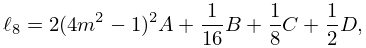
… ►and the coefficients ${\widetilde{𝒜}}_s(t)$ and ${\widetilde{ℬ}}_s(t)$ are given by … ►and the coefficients ${𝖠}_s(\tau )$ are the product of ${\tau }^s$ and a polynomial in $\tau$ of degree $2s$. …starting with ${𝖠}_0(\tau )=1$. … ►The coefficients $A_s(\zeta )$ and $B_s(\zeta )$ are given by …The coefficients $C_s(\zeta )$ and $D_s(\zeta )$ in (12.10.36) and (12.10.38) are given by …

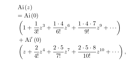
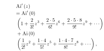
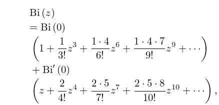
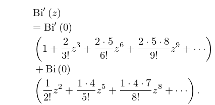
13: 9.4 Maclaurin Series

… ►

9.4.1 $$\mathrm{Ai}\left(z\right)=\mathrm{Ai}\left(0\right)\left(1+\frac{1}{3!}{z}^3+\frac{1\cdot 4}{6!}{z}^6+\frac{1\cdot 4\cdot 7}{9!}{z}^9+\mathrm{\cdots }\right)+{\mathrm{Ai}}^{\prime }\left(0\right)\left(z+\frac{2}{4!}{z}^4+\frac{2\cdot 5}{7!}{z}^7+\frac{2\cdot 5\cdot 8}{10!}{z}^{10}+\mathrm{\cdots }\right),$$

ⓘ

Symbols:

$\mathrm{Ai}\left(z\right)$: Airy function, $!$: factorial (as in $n!$) and $z$: complex variable

Source:

Olver (1997b, p. 54)

A&S Ref:

10.4.2 (with 10.4.4 and 10.4.5)

Permalink:

http://dlmf.nist.gov/9.4.E1

Encodings:

pMML, png, TeX

See also:

Annotations for §9.4 and Ch.9

►

9.4.2 $${\mathrm{Ai}}^{\prime }\left(z\right)={\mathrm{Ai}}^{\prime }\left(0\right)\left(1+\frac{2}{3!}{z}^3+\frac{2\cdot 5}{6!}{z}^6+\frac{2\cdot 5\cdot 8}{9!}{z}^9+\mathrm{\cdots }\right)+\mathrm{Ai}\left(0\right)\left(\frac{1}{2!}{z}^2+\frac{1\cdot 4}{5!}{z}^5+\frac{1\cdot 4\cdot 7}{8!}{z}^8+\mathrm{\cdots }\right),$$

ⓘ

Symbols:

$\mathrm{Ai}\left(z\right)$: Airy function, $!$: factorial (as in $n!$) and $z$: complex variable

Proof sketch:

Use methods of Olver (1997b, p. 54).

Permalink:

http://dlmf.nist.gov/9.4.E2

Encodings:

pMML, png, TeX

See also:

Annotations for §9.4 and Ch.9

►

9.4.3 $$\mathrm{Bi}\left(z\right)=\mathrm{Bi}\left(0\right)\left(1+\frac{1}{3!}{z}^3+\frac{1\cdot 4}{6!}{z}^6+\frac{1\cdot 4\cdot 7}{9!}{z}^9+\mathrm{\cdots }\right)+{\mathrm{Bi}}^{\prime }\left(0\right)\left(z+\frac{2}{4!}{z}^4+\frac{2\cdot 5}{7!}{z}^7+\frac{2\cdot 5\cdot 8}{10!}{z}^{10}+\mathrm{\cdots }\right),$$

ⓘ

Symbols:

$\mathrm{Bi}\left(z\right)$: Airy function, $!$: factorial (as in $n!$) and $z$: complex variable

Proof sketch:

Use methods of Olver (1997b, p. 54).

A&S Ref:

10.4.3 (with 10.4.4 and 10.4.5)

Referenced by:

(9.12.15)

Permalink:

http://dlmf.nist.gov/9.4.E3

Encodings:

pMML, png, TeX

See also:

Annotations for §9.4 and Ch.9

►

9.4.4 $${\mathrm{Bi}}^{\prime }\left(z\right)={\mathrm{Bi}}^{\prime }\left(0\right)\left(1+\frac{2}{3!}{z}^3+\frac{2\cdot 5}{6!}{z}^6+\frac{2\cdot 5\cdot 8}{9!}{z}^9+\mathrm{\cdots }\right)+\mathrm{Bi}\left(0\right)\left(\frac{1}{2!}{z}^2+\frac{1\cdot 4}{5!}{z}^5+\frac{1\cdot 4\cdot 7}{8!}{z}^8+\mathrm{\cdots }\right).$$

ⓘ

Symbols:

$\mathrm{Bi}\left(z\right)$: Airy function, $!$: factorial (as in $n!$) and $z$: complex variable

Proof sketch:

Use methods of Olver (1997b, p. 54).

Permalink:

http://dlmf.nist.gov/9.4.E4

Encodings:

pMML, png, TeX

See also:

Annotations for §9.4 and Ch.9

14: Bibliography

… ►

Tables of $\ln \mathrm{\Gamma }(z)$ for Complex Argument. Pergamon Press, New York.

ⓘ

External Links:

ZentralBlatt

Referenced by:

§5.22(iii).

Encodings:

BibTeX

… ►

Supplement to a paper “On the intensity of light in the neighbourhood of a caustic”. Trans. Camb. Phil. Soc. 8, pp. 595–599.

ⓘ

Referenced by:

§9.16.

Encodings:

BibTeX

… ►

Frequency response characteristics of the multiport planar elliptic patch. IEEE Trans. Microwave Theory Tech. 40 (8), pp. 1726–1730.

ⓘ

External Links:

Document

Referenced by:

6th item.

Encodings:

BibTeX

… ►

Algorithm 588. Fast Hankel transforms using related and lagged convolutions. ACM Trans. Math. Software 8 (4), pp. 369–370.

ⓘ

Notes:

Single-precision Fortran, maximum accuracy 8S.

External Links:

ISSN 0098-3500, Document, GAMS (module 588; package TOMS)

Referenced by:

2nd item.

Encodings:

BibTeX

… ►

Normal forms of functions near degenerate critical points, the Weyl groups $A_k,D_k,E_k$ and Lagrangian singularities. Funkcional. Anal. i Priložen. 6 (4), pp. 3–25 (Russian).

ⓘ

Notes:

In Russian. English translation: Functional Anal. Appl., 6(1973), pp. 254–272.

External Links:

MathReview (G. R. Belickii), ZentralBlatt

Referenced by:

§36.2(i).

Encodings:

BibTeX

…

15: 34.14 Tables

§34.14 Tables

►Tables of exact values of the squares of the $\mathit{3}j$ and $\mathit{6}j$ symbols in which all parameters are $\le 8$ are given in Rotenberg et al. (1959), together with a bibliography of earlier tables of $\mathit{3}j,\mathit{6}j$, and $\mathit{9}j$ symbols on pp. … ►Some selected $\mathit{9}j$ symbols are also given. … 16-17; for $\mathit{9}j$ symbols on p. … ► 310–332, and for the $\mathit{9}j$ symbols on pp. …

16: 10.41 Asymptotic Expansions for Large Order

… ►

$$U_{k+1}(p)=\frac{1}{2}{p}^2(1-p^2)U_k^{\prime }(p)+\frac{1}{8}{\int }_0^p(1-5t^2)U_k(t)dt,$$

… ►

$U_3(p)=\frac{1}{\mathrm{4\hspace{0.33em}14720}}(30375p^3-\mathrm{3\hspace{0.33em}69603}{p}^5+\mathrm{7\hspace{0.33em}65765}{p}^7-\mathrm{4\hspace{0.33em}25425}{p}^9),$

►

$V_1(p)=\frac{1}{24}(-9p+7p^3),$

… ►The curve $E_{1}B{E}_2$ in the $z$-plane is the upper boundary of the domain $𝐊$ depicted in Figure 10.20.3 and rotated through an angle $-\frac{1}{2}\pi$. … ►This is because $A_k(\zeta )$ and ${\zeta }^{-\frac{1}{2}}{B}_k(\zeta ),k=0,1,\mathrm{\dots }$, do not form an asymptotic scale (§2.1(v)) as $\zeta \to +\mathrm{\infty }$; see Olver (1997b, pp. 422–425). …

17: 24.2 Definitions and Generating Functions

… ►

Table 24.2.1: Bernoulli and Euler numbers.

► ►►►

$n$	$B_n$	$E_n$
…
$8$	$-\frac{1}{30}$	$1385$
…

►

… ►

Table 24.2.3: Bernoulli numbers $B_n=N/D$.

► ►►►

$n$	$N$	$D$	$B_n$
…
$8$	$-1$	$30$	$-\mathrm{3.33333\hspace{0.33em}3333}$	$\mathrm{\times 10⁻²}$
…

►

►

Table 24.2.4: Euler numbers $E_n$.

► ►►►

$n$	$E_n$
…
$8$	$1385$
…

►

►

Table 24.2.5: Coefficients $b_{n,k}$ of the Bernoulli polynomials $B_n\left(x\right)={\sum }_{k=0}^n{b}_{n,k}{x}^k$.

► ►►►

	$k$
$n$	$0$	$1$	$2$	$3$	$4$	$5$	$6$	$7$	$8$	$9$	$10$	$11$	$12$	$13$	$14$	$15$
…

►

►

Table 24.2.6: Coefficients $e_{n,k}$ of the Euler polynomials $E_n\left(x\right)={\sum }_{k=0}^n{e}_{n,k}{x}^k$.

► ►►►

	$k$
$n$	$0$	$1$	$2$	$3$	$4$	$5$	$6$	$7$	$8$	$9$	$10$	$11$	$12$	$13$	$14$	$15$
…

►

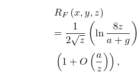
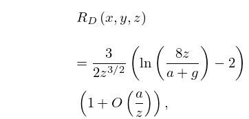
18: 19.27 Asymptotic Approximations and Expansions

… ►

§19.27(ii) $R_F(x,y,z)$

… ►

19.27.2 $$R_F(x,y,z)=\frac{1}{2\sqrt{z}}\left(\ln \frac{8z}{a+g}\right)\left(1+O\left(\frac{a}{z}\right)\right),$$ $a/z\to 0$.

ⓘ

Symbols:

$O\left(x\right)$: order not exceeding, $R_F(x,y,z)$: symmetric elliptic integral of first kind, $\ln z$: principal branch of logarithm function, $a$ and $g$

Referenced by:

§19.20(iii), §19.27(ii)

Permalink:

http://dlmf.nist.gov/19.27.E2

Encodings:

pMML, png, TeX

See also:

Annotations for §19.27(ii), §19.27 and Ch.19

… ►

19.27.6 $$R_G(0,y,z)=\frac{\sqrt{z}}{2}+\frac{y}{8\sqrt{z}}\left(\ln \left(\frac{16z}{y}\right)-1\right)\left(1+O\left(\frac{y}{z}\right)\right),$$ $y/z\to 0$.

ⓘ

Symbols:

$O\left(x\right)$: order not exceeding, $R_G(x,y,z)$: symmetric elliptic integral of second kind and $\ln z$: principal branch of logarithm function

Permalink:

http://dlmf.nist.gov/19.27.E6

Encodings:

pMML, png, TeX

See also:

Annotations for §19.27(iii), §19.27 and Ch.19

►

§19.27(iv) $R_D(x,y,z)$

… ►

19.27.7 $$R_D(x,y,z)=\frac{3}{2z^{3/2}}\left(\ln \left(\frac{8z}{a+g}\right)-2\right)\left(1+O\left(\frac{a}{z}\right)\right),$$ $a/z\to 0$.

ⓘ

Symbols:

$O\left(x\right)$: order not exceeding, $R_D(x,y,z)$: elliptic integral symmetric in only two variables, $\ln z$: principal branch of logarithm function, $a$ and $g$

Referenced by:

§19.20(iv)

Permalink:

http://dlmf.nist.gov/19.27.E7

Encodings:

pMML, png, TeX

See also:

Annotations for §19.27(iv), §19.27 and Ch.19

…

19: 19.29 Reduction of General Elliptic Integrals

… ►The advantages of symmetric integrals for tables of integrals and symbolic integration are illustrated by (19.29.4) and its cubic case, which replace the $8+8+12=28$ formulas in Gradshteyn and Ryzhik (2000, 3.147, 3.131, 3.152) after taking $x^2$ as the variable of integration in 3. …where the arguments of the $R_D$ function are, in order, $(a-b)(u-c)$, $(b-c)(a-u)$, $(a-b)(b-c)$. … ►The first choice gives a formula that includes the 18+9+18 = 45 formulas in Gradshteyn and Ryzhik (2000, 3.133, 3.156, 3.158), and the second choice includes the 8+8+8+12 = 36 formulas in Gradshteyn and Ryzhik (2000, 3.151, 3.149, 3.137, 3.157) (after setting $x^2=t$ in some cases). … ►where …(The variables of $R_F$ are real and nonnegative unless both $Q$’s have real zeros and those of $Q_1$ interlace those of $Q_2$.) …

20: 3.7 Ordinary Differential Equations

… ►where $f$, $g$, and $h$ are analytic functions in a domain $D\subset ℂ$. … ►Assume that we wish to integrate (3.7.1) along a finite path $𝒫$ from $z=a$ to $z=b$ in a domain $D$. The path is partitioned at $P+1$ points labeled successively $z_0,z_1,\mathrm{\dots },z_P$, with $z_0=a$, $z_P=b$. … ►where $𝐀(\tau ,z)$ is the matrix … ►Let ${𝐀}_P$ be the $(2P)\times (2P+2)$ band matrix …