%E5%8C%BA%E5%9D%97%E9%93%BE%E5%8D%9A%E5%BD%A9%E5%B9%B3%E5%8F%B0,%E5%8C%BA%E5%9D%97%E9%93%BE%E8%B5%8C%E5%9C%BA,%E5%8C%BA%E5%9D%97%E9%93%BE%E5%8D%9A%E5%BD%A9%E7%BD%91%E7%AB%99,%E3%80%90%E5%8C%BA%E5%9D%97%E9%93%BE%E5%8D%9A%E5%BD%A9%E5%9C%B0%E5%9D%80%E2%88%B633kk66.com%E3%80%91%E5%8C%BA%E5%9D%97%E9%93%BE%E8%B5%8C%E5%9C%BA,%E5%8C%BA%E5%9D%97%E9%93%BE%E5%8D%9A%E5%BD%A9%E9%A1%B9%E7%9B%AE,%E5%8E%BB%E4%B8%AD%E5%BF%83%E5%8C%96%E5%8D%9A%E5%BD%A9%E5%85%AC%E5%8F%B8,%E5%8C%BA%E5%9D%97%E9%93%BE%E6%B8%B8%E6%88%8F,%E5%8C%BA%E5%9D%97%E9%93%BE%E5%BD%A9%E7%A5%A8%E5%8C%BA%E5%9D%97%E9%93%BE%E5%8D%9A%E5%BD%A9%E5%B9%B3%E5%8F%B0%E3%80%90%E5%A4%8D%E5%88%B6%E6%89%93%E5%BC%80%E2%88%B633kk66.com%E3%80%91

SearchAdvancedHelp

(0.064 seconds)

11—20 of 783 matching pages

11: 21.5 Modular Transformations

… ►Let $𝐀$, $𝐁$, $𝐂$, and $𝐃$ be $g\times g$ matrices with integer elements such that …Here $\xi (𝚪)$ is an eighth root of unity, that is, ${(\xi (𝚪))}^8=1$. For general $𝚪$, it is difficult to decide which root needs to be used. … ►($𝐀$ invertible with integer elements.) …For a $g\times g$ matrix $𝐀$ we define $\mathrm{diag}𝐀$, as a column vector with the diagonal entries as elements. …

12: 32.9 Other Elementary Solutions

… ►with $C$ an arbitrary constant, which is solvable by quadrature. …${\text{P}}_{\text{III}}$ with $\alpha =\beta =\gamma =\delta =0$, has the general solution $w(z)=C{z}^{\mu }$, with $C$ and $\mu$ arbitrary constants. … ►

32.9.7 $$w(z;\mu ,-\frac{1}{8},-\mu {\kappa }^2,0)=1+\kappa z^{1/2},$$

ⓘ

Symbols:

$z$: real, $\kappa$: constant and $\mu$: constant

Permalink:

http://dlmf.nist.gov/32.9.E7

Encodings:

pMML, png, TeX

See also:

Annotations for §32.9(ii), §32.9 and Ch.32

… ►with $C$ an arbitrary constant, which is solvable by quadrature. …${\text{P}}_{\text{V}}$, with $\alpha =\beta =0$ and ${\gamma }^2+2\delta =0$, has solutions $w(z)=C\exp \left(\pm \sqrt{-2\delta }z\right)$, with $C$ an arbitrary constant. …

13: 33.10 Limiting Forms for Large $\rho$ or Large $\left|\eta \right|$

… ►

$F_{\mathrm{\ell }}(\eta ,\rho )\sim {\displaystyle \frac{(2\mathrm{\ell }+1)!C_{\mathrm{\ell }}\left(\eta \right)}{{(2\eta )}^{\mathrm{\ell }+1}}}{(2\eta \rho )}^{1/2}{I}_{2\mathrm{\ell }+1}\left({(8\eta \rho )}^{1/2}\right),$

►

$G_{\mathrm{\ell }}(\eta ,\rho )\sim {\displaystyle \frac{2{(2\eta )}^{\mathrm{\ell }}}{(2\mathrm{\ell }+1)!C_{\mathrm{\ell }}\left(\eta \right)}}{(2\eta \rho )}^{1/2}{K}_{2\mathrm{\ell }+1}\left({(8\eta \rho )}^{1/2}\right).$

… ►

$$F_0(\eta ,\rho )\sim {\mathrm{e}}^{-\pi \eta }{(\pi \rho )}^{1/2}{I}_1\left({(8\eta \rho )}^{1/2}\right),$$

… ►

$$F_{\mathrm{\ell }}(\eta ,\rho )=\frac{(2\mathrm{\ell }+1)!C_{\mathrm{\ell }}\left(\eta \right)}{{(-2\eta )}^{\mathrm{\ell }+1}}\left({(-2\eta \rho )}^{1/2}{J}_{2\mathrm{\ell }+1}\left({(-8\eta \rho )}^{1/2}\right)+o\left({\left|\eta \right|}^{1/4}\right)\right),$$

►

$$G_{\mathrm{\ell }}(\eta ,\rho )=-\frac{\pi {(-2\eta )}^{\mathrm{\ell }}}{(2\mathrm{\ell }+1)!C_{\mathrm{\ell }}\left(\eta \right)}\left({(-2\eta \rho )}^{1/2}{Y}_{2\mathrm{\ell }+1}\left({(-8\eta \rho )}^{1/2}\right)+o\left({\left|\eta \right|}^{1/4}\right)\right).$$

…

14: 18.8 Differential Equations

… ►

Table 18.8.1: Classical OP’s: differential equations $A(x)f^{\prime \prime }(x)+B(x)f^{\prime }(x)+C(x)f(x)+{\lambda }_{n}f(x)=0$.

► ►►►►►

#	$f(x)$	$A(x)$	$B(x)$	$C(x)$	${\lambda }_n$
…
4	$C_n^{(\lambda )}\left(x\right)$	$1-x^2$	$-(2\lambda +1)x$	$0$	$n(n+2\lambda )$
…
8	$L_n^{(\alpha )}\left(x\right)$	$x$	$\alpha +1-x$	$0$	$n$
9	${\mathrm{e}}^{-\frac{1}{2}{x}^2}{x}^{\alpha +\frac{1}{2}}{L}_n^{(\alpha )}\left(x^2\right)$	$1$	$0$	$-x^2+(\frac{1}{4}-{\alpha }^2)x^{-2}$	$4n+2\alpha +2$
…

►

…

15: 9.4 Maclaurin Series

… ►

9.4.1 $$\mathrm{Ai}\left(z\right)=\mathrm{Ai}\left(0\right)\left(1+\frac{1}{3!}{z}^3+\frac{1\cdot 4}{6!}{z}^6+\frac{1\cdot 4\cdot 7}{9!}{z}^9+\mathrm{\cdots }\right)+{\mathrm{Ai}}^{\prime }\left(0\right)\left(z+\frac{2}{4!}{z}^4+\frac{2\cdot 5}{7!}{z}^7+\frac{2\cdot 5\cdot 8}{10!}{z}^{10}+\mathrm{\cdots }\right),$$

ⓘ

Symbols:

$\mathrm{Ai}\left(z\right)$: Airy function, $!$: factorial (as in $n!$) and $z$: complex variable

Source:

Olver (1997b, p. 54)

A&S Ref:

10.4.2 (with 10.4.4 and 10.4.5)

Permalink:

http://dlmf.nist.gov/9.4.E1

Encodings:

pMML, png, TeX

See also:

Annotations for §9.4 and Ch.9

►

9.4.2 $${\mathrm{Ai}}^{\prime }\left(z\right)={\mathrm{Ai}}^{\prime }\left(0\right)\left(1+\frac{2}{3!}{z}^3+\frac{2\cdot 5}{6!}{z}^6+\frac{2\cdot 5\cdot 8}{9!}{z}^9+\mathrm{\cdots }\right)+\mathrm{Ai}\left(0\right)\left(\frac{1}{2!}{z}^2+\frac{1\cdot 4}{5!}{z}^5+\frac{1\cdot 4\cdot 7}{8!}{z}^8+\mathrm{\cdots }\right),$$

ⓘ

Symbols:

$\mathrm{Ai}\left(z\right)$: Airy function, $!$: factorial (as in $n!$) and $z$: complex variable

Proof sketch:

Use methods of Olver (1997b, p. 54).

Permalink:

http://dlmf.nist.gov/9.4.E2

Encodings:

pMML, png, TeX

See also:

Annotations for §9.4 and Ch.9

►

9.4.3 $$\mathrm{Bi}\left(z\right)=\mathrm{Bi}\left(0\right)\left(1+\frac{1}{3!}{z}^3+\frac{1\cdot 4}{6!}{z}^6+\frac{1\cdot 4\cdot 7}{9!}{z}^9+\mathrm{\cdots }\right)+{\mathrm{Bi}}^{\prime }\left(0\right)\left(z+\frac{2}{4!}{z}^4+\frac{2\cdot 5}{7!}{z}^7+\frac{2\cdot 5\cdot 8}{10!}{z}^{10}+\mathrm{\cdots }\right),$$

ⓘ

Symbols:

$\mathrm{Bi}\left(z\right)$: Airy function, $!$: factorial (as in $n!$) and $z$: complex variable

Proof sketch:

Use methods of Olver (1997b, p. 54).

A&S Ref:

10.4.3 (with 10.4.4 and 10.4.5)

Referenced by:

(9.12.15)

Permalink:

http://dlmf.nist.gov/9.4.E3

Encodings:

pMML, png, TeX

See also:

Annotations for §9.4 and Ch.9

►

9.4.4 $${\mathrm{Bi}}^{\prime }\left(z\right)={\mathrm{Bi}}^{\prime }\left(0\right)\left(1+\frac{2}{3!}{z}^3+\frac{2\cdot 5}{6!}{z}^6+\frac{2\cdot 5\cdot 8}{9!}{z}^9+\mathrm{\cdots }\right)+\mathrm{Bi}\left(0\right)\left(\frac{1}{2!}{z}^2+\frac{1\cdot 4}{5!}{z}^5+\frac{1\cdot 4\cdot 7}{8!}{z}^8+\mathrm{\cdots }\right).$$

ⓘ

Symbols:

$\mathrm{Bi}\left(z\right)$: Airy function, $!$: factorial (as in $n!$) and $z$: complex variable

Proof sketch:

Use methods of Olver (1997b, p. 54).

Permalink:

http://dlmf.nist.gov/9.4.E4

Encodings:

pMML, png, TeX

See also:

Annotations for §9.4 and Ch.9

16: 28.8 Asymptotic Expansions for Large $q$

… ►Also let $\xi =2\sqrt{h}\cos x$ and $D_m\left(\xi \right)={\mathrm{e}}^{-{\xi }^2/4}{\mathrm{𝐻𝑒}}_m\left(\xi \right)$ (§18.3). … ►

28.8.4 $$U_m(\xi )\sim D_m\left(\xi \right)-\frac{1}{2^{6}h}\left(D_{m+4}\left(\xi \right)-4!\left(\genfrac{}{}{0pt}{}{m}{4}\right)D_{m-4}\left(\xi \right)\right)+\frac{1}{2^{13}{h}^2}\left(D_{m+8}\left(\xi \right)-2^5(m+2)D_{m+4}\left(\xi \right)+4!{\mathrm{\hspace{0.17em}2}}^5(m-1)\left(\genfrac{}{}{0pt}{}{m}{4}\right)D_{m-4}\left(\xi \right)+8!\left(\genfrac{}{}{0.0pt}{}{m}{8}\right)D_{m-8}\left(\xi \right)\right)+\mathrm{\cdots },$$

ⓘ

Defines:

$U_m(\xi )$: function (locally)

Symbols:

$D_{\nu }\left(z\right)$: parabolic cylinder function, $\sim$: Poincaré asymptotic expansion, $\left(\genfrac{}{}{0.0pt}{}{m}{n}\right)$: binomial coefficient, $!$: factorial (as in $n!$), $m$: integer, $h$: parameter and $\xi$: variable

A&S Ref:

20.9.17 (in different form)

Permalink:

http://dlmf.nist.gov/28.8.E4

Encodings:

pMML, png, TeX

See also:

Annotations for §28.8(ii), §28.8 and Ch.28

… ►

28.8.6 $${\widehat{C}}_m\sim {\left(\frac{\pi h}{2{(m!)}^2}\right)}^{1/4}{\left(1+\frac{2m+1}{8h}+\frac{m^4+2m^3+263m^2+262m+108}{2048h^2}+\mathrm{\cdots }\right)}^{-1/2},$$

ⓘ

Defines:

${\widehat{C}}_m$: coefficient (locally)

Symbols:

$\sim$: Poincaré asymptotic expansion, $\pi$: the ratio of the circumference of a circle to its diameter, $!$: factorial (as in $n!$), $m$: integer and $h$: parameter

A&S Ref:

20.9.19 (in slightly different form)

Permalink:

http://dlmf.nist.gov/28.8.E6

Encodings:

pMML, png, TeX

See also:

Annotations for §28.8(ii), §28.8 and Ch.28

►

28.8.7 $${\widehat{S}}_m\sim {\left(\frac{\pi h}{2{(m!)}^2}\right)}^{1/4}{\left(1-\frac{2m+1}{8h}+\frac{m^4+2m^3-121m^2-122m-84}{2048h^2}+\mathrm{\cdots }\right)}^{-1/2}.$$

ⓘ

Defines:

${\widehat{S}}_m$: coefficient (locally)

Symbols:

$\sim$: Poincaré asymptotic expansion, $\pi$: the ratio of the circumference of a circle to its diameter, $!$: factorial (as in $n!$), $m$: integer and $h$: parameter

A&S Ref:

20.9.20 (in slightly different form)

Referenced by:

§28.8(ii), Erratum (V1.1.10) for Sections 28.6(i), 28.6(ii), 28.8(i), 28.8(ii)

Permalink:

http://dlmf.nist.gov/28.8.E7

Encodings:

pMML, png, TeX

See also:

Annotations for §28.8(ii), §28.8 and Ch.28

… ►It is stated that corresponding uniform approximations can be obtained for other solutions, including the eigensolutions, of the differential equations by application of the results, but these approximations are not included. …

17: 19.36 Methods of Computation

… ►If (19.36.1) is used instead of its first five terms, then the factor ${(3r)}^{-1/6}$ in Carlson (1995, (2.2)) is changed to ${(3r)}^{-1/8}$. ►For both $R_D$ and $R_J$ the factor ${(r/4)}^{-1/6}$ in Carlson (1995, (2.18)) is changed to ${(r/5)}^{-1/8}$ when the following polynomial of degree 7 (the same for both) is used instead of its first seven terms: … ►All cases of $R_F$, $R_C$, $R_J$, and $R_D$ are computed by essentially the same procedure (after transforming Cauchy principal values by means of (19.20.14) and (19.2.20)). … ►The step from $n$ to $n+1$ is an ascending Landen transformation if $\theta =1$ (leading ultimately to a hyperbolic case of $R_C$) or a descending Gauss transformation if $\theta =-1$ (leading to a circular case of $R_C$). … ►Here $R_C$ is computed either by the duplication algorithm in Carlson (1995) or via (19.2.19). …

18: 19.17 Graphics

… ►For $R_F$, $R_G$, and $R_J$, which are symmetric in $x,y,z$, we may further assume that $z$ is the largest of $x,y,z$ if the variables are real, then choose $z=1$, and consider only $0\le x\le 1$ and $0\le y\le 1$. … ►To view $R_F(0,y,1)$ and $2R_G(0,y,1)$ for complex $y$, put $y=1-k^2$, use (19.25.1), and see Figures 19.3.7–19.3.12. … ►To view $R_F(0,y,1)$ and $2R_G(0,y,1)$ for complex $y$, put $y=1-k^2$, use (19.25.1), and see Figures 19.3.7–19.3.12. … ►

►►

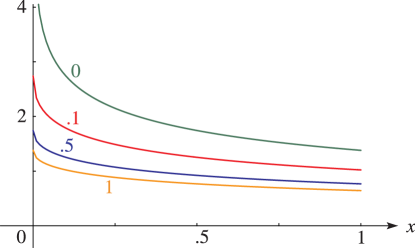
Figure 19.17.4: $R_J(x,y,1,2)$ for $0\le x\le 1$, $y=0,\mathrm{\hspace{0.17em}0.1},\mathrm{\hspace{0.17em}0.5},\mathrm{\hspace{0.17em}1}$. $y=1$ corresponds to $3(R_C(x,1)-R_C(x,2))$. Magnify

… ►

►►

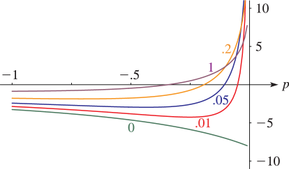
Figure 19.17.7: Cauchy principal value of $R_J(0.5,y,1,p)$ for $y=0,\mathrm{\hspace{0.17em}0.01},\mathrm{\hspace{0.17em}0.05},\mathrm{\hspace{0.17em}0.2},\mathrm{\hspace{0.17em}1}$, . $y=1$ corresponds to $3(R_C(0.5,p)-(\pi /\sqrt{8}))/(1-p)$. … Magnify

…

19: 27.2 Functions

… ►($\nu \left(1\right)$ is defined to be 0.) …It can be expressed as a sum over all primes $p\le x$: … ►It is the special case $k=2$ of the function $d_k\left(n\right)$ that counts the number of ways of expressing $n$ as the product of $k$ factors, with the order of factors taken into account. …Note that ${\sigma }_0\left(n\right)=d\left(n\right)$. … ►Table 27.2.2 tabulates the Euler totient function $\varphi \left(n\right)$, the divisor function $d\left(n\right)$ ($={\sigma }_0(n)$), and the sum of the divisors $\sigma (n)$ ($={\sigma }_1(n)$), for $n=1(1)52$. …

20: 19.26 Addition Theorems

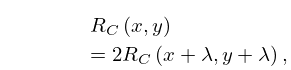
… ►In this subsection, and also §§19.26(ii) and 19.26(iii), we assume that $\lambda ,x,y,z$ are positive, except that at most one of $x,y,z$ can be 0. …where for $\gamma =\alpha ,\beta ,\sigma$, except that ${\sigma }^2-\theta$ can be 0, and … ►An equivalent version for $R_C$ is … ►either upper or lower signs being taken throughout. … ►

19.26.25 $$R_C(x,y)=2R_C(x+\lambda ,y+\lambda ),$$ $\lambda =y+2\sqrt{x}\sqrt{y}$.

ⓘ

Symbols:

$R_C(x,y)$: Carlson’s combination of inverse circular and inverse hyperbolic functions, $\lambda$: positive, $x$: positive and $y$: positive

Referenced by:

§19.26(iii)

Permalink:

http://dlmf.nist.gov/19.26.E25

Encodings:

pMML, png, TeX

See also:

Annotations for §19.26(iii), §19.26 and Ch.19

…