as eigenfunctions of a q-difference operator

SearchAdvancedHelp

(0.005 seconds)

41—50 of 892 matching pages

41: 17.2 Calculus

… ► … ►Note that (17.2.6_1) is just (27.14.14) with $a=d=0$ and $-b=c=1$. … ►When $a=q^{m+1}$, where $m$ is a nonnegative integer, (17.2.37) reduces to the $q$-binomial series … ►If $f(x)$ is continuous on $[0,a]$, then … ►These identities are the first in a large collection of similar results. …

42: 30.4 Functions of the First Kind

… ►The eigenfunctions of (30.2.1) that correspond to the eigenvalues ${\lambda }_n^m\left({\gamma }^2\right)$ are denoted by ${\mathrm{𝖯𝗌}}_n^m(x,{\gamma }^2)$, $n=m,m+1,m+2,\mathrm{\dots }$. …

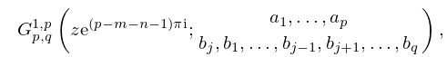
43: 18.1 Notation

… ►

$x$-Differences

►Forward differences: … ►Backward differences: … ►Central differences in imaginary direction: … ►In Koekoek et al. (2010) ${\delta }_x$ denotes the operator $\mathrm{i}{\delta }_x$.

44: Philip J. Davis

… ►He returned to Harvard after the war and completed a Ph. … ►At that time John Todd was Chief of the Numerical Analysis Section of the Applied Mathematics Division and head of the Computation Laboratory that co-developed, with the NBS Electronic Computer Laboratory, the Standards Eastern Automatic Computer (SEAC), the first fully operational stored-program electronic digital computer in the United States. … ►” Davis believed it was the first chapter written, and he laid out a schema that could serve as a model for the other chapters. Davis also co-authored a second Chapter, “Numerical Interpolation, Differentiation, and Integration” with Ivan Polonsky. … ►Moreover, a cutting plane feature allows users to track curves of intersection produced as a moving plane cuts through the function surface. …

45: 1.4 Calculus of One Variable

… ►A function $f(x)$ is square-integrable if … ►If , then $f(x)$ is of bounded variation on $(a,b)$. In this case, $g(x)={𝒱}_{a,x}\left(f\right)$ and $h(x)={𝒱}_{a,x}\left(f\right)-f(x)$ are nondecreasing bounded functions and $f(x)=g(x)-h(x)$. … ►Lastly, whether or not the real numbers $a$ and $b$ satisfy , and whether or not they are finite, we define ${𝒱}_{a,b}\left(f\right)$ by (1.4.34) whenever this integral exists. … ►A function $f(x)$ is convex on $(a,b)$ if …

46: 16.21 Differential Equation

… ► $w=G_{p,q}^{m,n}(z;𝐚;𝐛)$ satisfies the differential equation ►

16.21.1 $$\left({(-1)}^{p-m-n}z(\mathit{\vartheta }-a_1+1)\mathrm{\cdots }(\mathit{\vartheta }-a_p+1)-(\mathit{\vartheta }-b_1)\mathrm{\cdots }(\mathit{\vartheta }-b_q)\right)w=0,$$

ⓘ

Symbols:

$p$: nonnegative integer, $q$: nonnegative integer, $z$: complex variable, $a,a_1,\mathrm{\dots },a_p$: real or complex parameters, $b,b_1,\mathrm{\dots },b_q$: real or complex parameters, $w$: solution and $\mathit{\vartheta }$: differential operator

Referenced by:

§16.21, §16.21

Permalink:

http://dlmf.nist.gov/16.21.E1

Encodings:

pMML, png, TeX

See also:

Annotations for §16.21 and Ch.16

… ►With the classification of §16.8(i), when the only singularities of (16.21.1) are a regular singularity at $z=0$ and an irregular singularity at $z=\mathrm{\infty }$. … ►A fundamental set of solutions of (16.21.1) is given by ►

16.21.2 $$G_{p,q}^{1,p}(z{\mathrm{e}}^{(p-m-n-1)\pi \mathrm{i}};\genfrac{}{}{0pt}{}{a_1,\mathrm{\dots },a_p}{b_j,b_1,\mathrm{\dots },b_{j-1},b_{j+1},\mathrm{\dots },b_q}),$$ $j=1,\mathrm{\dots },q$.

ⓘ

Symbols:

$G_{p,q}^{m,n}(z;\genfrac{}{}{0pt}{}{a_1,\mathrm{\dots },a_p}{b_1,\mathrm{\dots },b_q})$ or $G_{p,q}^{m,n}(z;𝐚;𝐛)$: Meijer $G$-function, $\pi$: the ratio of the circumference of a circle to its diameter, $\mathrm{e}$: base of natural logarithm, $\mathrm{i}$: imaginary unit, $p$: nonnegative integer, $q$: nonnegative integer, $z$: complex variable, $a,a_1,\mathrm{\dots },a_p$: real or complex parameters and $b,b_1,\mathrm{\dots },b_q$: real or complex parameters

Permalink:

http://dlmf.nist.gov/16.21.E2

Encodings:

pMML, png, TeX

See also:

Annotations for §16.21 and Ch.16

…

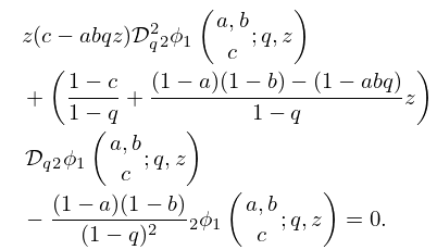
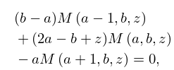
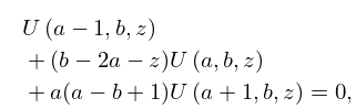
47: 17.6 ${}_2{}^{}\varphi _1^{}$ Function

… ►For a similar result for $q$-confluent hypergeometric functions see Morita (2013). … ►

Iterations of $𝒟$

… ►

17.6.27 $$z(c-abqz){𝒟}_q^2{}_2{}^{}\varphi _1^{}(\genfrac{}{}{0pt}{}{a,b}{c};q,z)+\left(\frac{1-c}{1-q}+\frac{(1-a)(1-b)-(1-abq)}{1-q}z\right){𝒟}_q{}_2{}^{}\varphi _1^{}(\genfrac{}{}{0pt}{}{a,b}{c};q,z)-\frac{(1-a)(1-b)}{{(1-q)}^2}{}_2{}^{}\varphi _1^{}(\genfrac{}{}{0pt}{}{a,b}{c};q,z)=0.$$

ⓘ

Symbols:

${}_{r+1}{}^{}\varphi _s^{}(a_0,\mathrm{\dots },a_r;b_1,\mathrm{\dots },b_s;q,z)$ or ${}_{r+1}{}^{}\varphi _s^{}(\genfrac{}{}{0pt}{}{a_0,\mathrm{\dots },a_r}{b_1,\mathrm{\dots },b_s};q,z)$: basic hypergeometric (or $q$-hypergeometric) function, $q$: complex base, $z$: complex variable and ${𝒟}_q$: $q$-differential operator

Referenced by:

§17.6(iv)

Permalink:

http://dlmf.nist.gov/17.6.E27

Encodings:

pMML, png, TeX

See also:

Annotations for §17.6(iv), §17.6(iv), §17.6 and Ch.17

►(17.6.27) reduces to the hypergeometric equation (15.10.1) with the substitutions $a\to q^a$, $b\to q^b$, $c\to q^c$, followed by ${lim}_{q\to 1-}$. … ►where , , and the contour of integration separates the poles of ${(q^{1+\zeta },c{q}^{\zeta };q)}_{\mathrm{\infty }}/\sin \left(\pi \zeta \right)$ from those of $1/{(a{q}^{\zeta },b{q}^{\zeta };q)}_{\mathrm{\infty }}$, and the infimum of the distances of the poles from the contour is positive. …

48: 1.15 Summability Methods

… ►(Here and elsewhere in this subsection $\delta$ is a constant such that .) … ► $A(r,\theta )$ is a harmonic function in polar coordinates (1.9.27), and … ►The lower limit $0$ of the integral in (1.15.47) can be replaced by any constant $a\le x$ . Also, we can replace the lower and upper limits of the integral by $x$ and $a$, respectively. … ►and either $\left|a_n\right|\le K$ or $a_n\ge 0$, then …

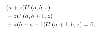
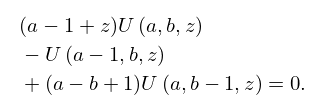
49: 13.3 Recurrence Relations and Derivatives

… ►

13.3.1 $$(b-a)M(a-1,b,z)+(2a-b+z)M(a,b,z)-aM(a+1,b,z)=0,$$

ⓘ

Symbols:

$M(a,b,z)$: $={}_1{}^{}F_1^{}(a;b;z)$ Kummer confluent hypergeometric function and $z$: complex variable

A&S Ref:

13.4.1

Permalink:

http://dlmf.nist.gov/13.3.E1

Encodings:

pMML, png, TeX

See also:

Annotations for §13.3(i), §13.3 and Ch.13

… ►

13.3.7 $$U(a-1,b,z)+(b-2a-z)U(a,b,z)+a(a-b+1)U(a+1,b,z)=0,$$

ⓘ

Symbols:

$U(a,b,z)$: Kummer confluent hypergeometric function and $z$: complex variable

A&S Ref:

13.4.15

Permalink:

http://dlmf.nist.gov/13.3.E7

Encodings:

pMML, png, TeX

See also:

Annotations for §13.3(i), §13.3 and Ch.13

… ►

13.3.11 $$(a+z)U(a,b,z)-zU(a,b+1,z)+a(b-a-1)U(a+1,b,z)=0,$$

ⓘ

Symbols:

$U(a,b,z)$: Kummer confluent hypergeometric function and $z$: complex variable

A&S Ref:

13.4.19

Permalink:

http://dlmf.nist.gov/13.3.E11

Encodings:

pMML, png, TeX

See also:

Annotations for §13.3(i), §13.3 and Ch.13

►

13.3.12 $$(a-1+z)U(a,b,z)-U(a-1,b,z)+(a-b+1)U(a,b-1,z)=0.$$

ⓘ

Symbols:

$U(a,b,z)$: Kummer confluent hypergeometric function and $z$: complex variable

A&S Ref:

13.4.20

Permalink:

http://dlmf.nist.gov/13.3.E12

Encodings:

pMML, png, TeX

See also:

Annotations for §13.3(i), §13.3 and Ch.13

… ►Other versions of several of the identities in this subsection can be constructed with the aid of the operator identity …

50: 10.17 Asymptotic Expansions for Large Argument

… ►Define $a_0(\nu )=1$, … ►Similarly for ${\sum }_{k=0}^{\mathrm{\ell }-1}{(-1)}^k{a}_{2k+1}(\nu )z^{-2k-1}$, provided that $\mathrm{\ell }\ge \max (\frac{1}{2}\nu -\frac{3}{4},1)$. … ►where $𝒱$ denotes the variational operator (2.3.6), and the paths of variation are subject to the condition that $|\mathrm{\Im }t|$ changes monotonically. Bounds for ${𝒱}_{z,\mathrm{i}\mathrm{\infty }}\left(t^{-\mathrm{\ell }}\right)$ are given by … ►The bounds (10.17.15) also apply to ${𝒱}_{z,-\mathrm{i}\mathrm{\infty }}\left(t^{-\mathrm{\ell }}\right)$ in the conjugate sectors. …