small%20k%2Ck%E2%80%B2

SearchAdvancedHelp

(0.005 seconds)

1—10 of 832 matching pages

1: 26.6 Other Lattice Path Numbers

… ► $M(n)$ is the number of lattice paths from $(0,0)$ to $(n,n)$ that stay on or above the line $y=x$ and are composed of directed line segments of the form $(2,0)$, $(0,2)$, or $(1,1)$. … ►

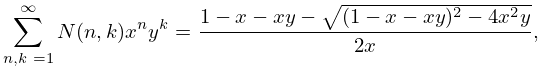
Narayana Number $N(n,k)$

► $N(n,k)$ is the number of lattice paths from $(0,0)$ to $(n,n)$ that stay on or above the line $y=x$, are composed of directed line segments of the form $(1,0)$ or $(0,1)$, and for which there are exactly $k$ occurrences at which a segment of the form $(0,1)$ is followed by a segment of the form $(1,0)$. … ►For sufficiently small $|x|$ and $|y|$, … ►

26.6.8 $$\sum _{n,k=1}^{\mathrm{\infty }}N(n,k)x^n{y}^k=\frac{1-x-xy-\sqrt{{(1-x-xy)}^2-4x^{2}y}}{2x},$$

ⓘ

Symbols:

$k$: nonnegative integer, $n$: nonnegative integer, $N(n,k)$: Narayana number, $x$: small and $y$: small

Permalink:

http://dlmf.nist.gov/26.6.E8

Encodings:

pMML, png, TeX

See also:

Annotations for §26.6(ii), §26.6 and Ch.26

…

2: 10.75 Tables

… ►

British Association for the Advancement of Science (1937) tabulates $I_0\left(x\right)$, $I_1\left(x\right)$, $x=0(.001)5$, 7–8D; $K_0\left(x\right)$, $K_1\left(x\right)$, $x=0.01(.01)5$, 7–10D; ${\mathrm{e}}^{-x}{I}_0\left(x\right)$, ${\mathrm{e}}^{-x}{I}_1\left(x\right)$, ${\mathrm{e}}^x{K}_0\left(x\right)$, ${\mathrm{e}}^x{K}_1\left(x\right)$, $x=5(.01)10(.1)20$, 8D. Also included are auxiliary functions to facilitate interpolation of the tables of $K_0\left(x\right)$, $K_1\left(x\right)$ for small values of $x$.

►

Bickley et al. (1952) tabulates $x^{-n}{I}_n\left(x\right)$ or ${\mathrm{e}}^{-x}{I}_n\left(x\right)$, $x^n{K}_n\left(x\right)$ or ${\mathrm{e}}^x{K}_n\left(x\right)$, $n=2(1)20$, $x=0$(.01 or .1) 10(.1) 20, 8S; $I_n\left(x\right)$, $K_n\left(x\right)$, $n=0(1)20$, $x=0$ or $0.1(.1)20$, 10S.

… ►

The main tables in Abramowitz and Stegun (1964, Chapter 9) give ${\mathrm{e}}^{-x}{I}_n\left(x\right)$, ${\mathrm{e}}^x{K}_n\left(x\right)$, $n=0,1,2$, $x=0(.1)10(.2)20$, 8D–10D or 10S; $\sqrt{x}{\mathrm{e}}^{-x}{I}_n\left(x\right)$, $(\sqrt{x}/\pi )$ ${\mathrm{e}}^x{K}_n\left(x\right)$, $n=0,1,2$, $1/x=0(.002)0.05$; $K_0\left(x\right)+I_0\left(x\right)\ln x$, $x(K_1\left(x\right)-I_1\left(x\right)\ln x)$, $x=0(.1)2$, 8D; ${\mathrm{e}}^{-x}{I}_n\left(x\right)$, ${\mathrm{e}}^x{K}_n\left(x\right)$, $n=3(1)9$, $x=0(.2)10(.5)20$, 5S; $I_n\left(x\right)$, $K_n\left(x\right)$, $n=0(1)20(10)50,100$, $x=1,2,5,10,50,100$, 9–10S.

… ►

Kerimov and Skorokhodov (1984b) tabulates all zeros of the principal values of $K_n\left(z\right)$ and $K_n^{\prime }\left(z\right)$, for $n=2(1)20$, 9S.

… ►

The main tables in Abramowitz and Stegun (1964, Chapter 10) give ${𝗃}_n\left(x\right)$, ${𝗒}_n\left(x\right)$ $n=0(1)8$, $x=0(.1)10$, 5–8S; ${𝗃}_n\left(x\right)$, ${𝗒}_n\left(x\right)$ $n=0(1)20(10)50$, 100, $x=1,2,5,10,50,100$, 10S; ${𝗂}_n^{(1)}\left(x\right)$, ${𝗄}_n\left(x\right)$, $n=0,1,2$, $x=0(.1)5$, 4–9D; ${𝗂}_n^{(1)}\left(x\right)$, ${𝗄}_n\left(x\right)$, $n=0(1)20(10)50$, 100, $x=1,2,5,10,50,100$, 10S. (For the notation see §10.1 and §10.47(ii).)

…

3: 11.6 Asymptotic Expansions

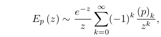
… ►where $\delta$ is an arbitrary small positive constant. If the series on the right-hand side of (11.6.1) is truncated after $m(\ge 0)$ terms, then the remainder term $R_m(z)$ is $O\left(z^{\nu -2m-1}\right)$. If $\nu$ is real, $z$ is positive, and $m+\frac{1}{2}-\nu \ge 0$, then $R_m(z)$ is of the same sign and numerically less than the first neglected term. … ►Here …These and higher coefficients $c_k(\lambda )$ can be computed via the representations in Nemes (2015b). …

4: 9.7 Asymptotic Expansions

… ►Here $\delta$ denotes an arbitrary small positive constant and …Also $u_0=v_0=1$ and for $k=1,2,\mathrm{\dots }$, … ►Numerical values of $\chi (n)$ are given in Table 9.7.1 for $n=1(1)20$ to 2D. … ►where $\xi =\frac{2}{3}{x}^{3/2}$. … ►with $n=\lfloor 2|\zeta |\rfloor$. …

5: 36.5 Stokes Sets

… ►Stokes sets are surfaces (codimension one) in $𝐱$ space, across which ${\mathrm{\Psi }}_K(𝐱;k)$ or ${\mathrm{\Psi }}^{(\mathrm{U})}(𝐱;k)$ acquires an exponentially-small asymptotic contribution (in $k$), associated with a complex critical point of ${\mathrm{\Phi }}_K$ or . … ►

$K=1$. Airy Function

… ►

$K=2$. Cusp

… ►

$K=3$. Swallowtail

… ►For , there are two solutions $u$, provided that $|Y|>{(\frac{2}{5})}^{1/2}$. …

6: 33.5 Limiting Forms for Small $\rho$, Small $|\eta |$, or Large $\mathrm{\ell }$

§33.5 Limiting Forms for Small $\rho$, Small $|\eta |$, or Large $\mathrm{\ell }$

►

§33.5(i) Small $\rho$

… ►

$$F_{\mathrm{\ell }}(0,\rho )={(\pi \rho /2)}^{1/2}{J}_{\mathrm{\ell }+\frac{1}{2}}\left(\rho \right),$$

►

$$G_{\mathrm{\ell }}(0,\rho )=-{(\pi \rho /2)}^{1/2}{Y}_{\mathrm{\ell }+\frac{1}{2}}\left(\rho \right).$$

… ►

§33.5(iii) Small $|\eta |$

…

7: 11.1 Special Notation

… ► ►►►►

$x$	real variable.
…
$k$	nonnegative integer.
$\delta$	arbitrary small positive constant.

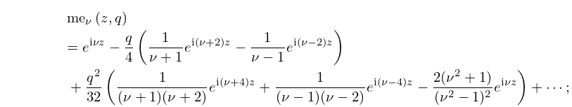
… ►For the functions $J_{\nu }\left(z\right)$, $Y_{\nu }\left(z\right)$, $H_{\nu }^{(1)}\left(z\right)$, $H_{\nu }^{(2)}\left(z\right)$, $I_{\nu }\left(z\right)$, and $K_{\nu }\left(z\right)$ see §§10.2(ii), 10.25(ii). ►The functions treated in this chapter are the Struve functions ${𝐇}_{\nu }\left(z\right)$ and ${𝐊}_{\nu }\left(z\right)$, the modified Struve functions ${𝐋}_{\nu }\left(z\right)$ and ${𝐌}_{\nu }\left(z\right)$, the Lommel functions $s_{\mu ,\nu }\left(z\right)$ and $S_{\mu ,\nu }\left(z\right)$, the Anger function ${𝐉}_{\nu }\left(z\right)$, the Weber function ${𝐄}_{\nu }\left(z\right)$, and the associated Anger–Weber function ${𝐀}_{\nu }\left(z\right)$.

8: 12.1 Special Notation

… ► ►►►

$x,y$	real variables.
…
$\delta$	arbitrary small positive constant.

… ►The notations are related by $U(a,z)=D_{-a-\frac{1}{2}}\left(z\right)$. …

9: 8.20 Asymptotic Expansions of $E_p\left(z\right)$

… ►

8.20.2 $$E_p\left(z\right)\sim \frac{{\mathrm{e}}^{-z}}{z}\sum _{k=0}^{\mathrm{\infty }}{(-1)}^k\frac{{\left(p\right)}_k}{z^k},$$ $|\mathrm{ph}z|\le \frac{3}{2}\pi -\delta$,

ⓘ

Symbols:

${\left(a\right)}_n$: Pochhammer’s symbol (or shifted factorial), $\sim$: Poincaré asymptotic expansion, $\pi$: the ratio of the circumference of a circle to its diameter, $\mathrm{e}$: base of natural logarithm, $E_p\left(z\right)$: generalized exponential integral, $\mathrm{ph}$: phase, $z$: complex variable, $p$: parameter, $k$: nonnegative integer and $\delta$: small positive constant

Referenced by:

§8.20(i)

Permalink:

http://dlmf.nist.gov/8.20.E2

Encodings:

pMML, png, TeX

See also:

Annotations for §8.20(i), §8.20 and Ch.8

… ► $\delta$ again denoting an arbitrary small positive constant. Where the sectors of validity of (8.20.2) and (8.20.3) overlap the contribution of the first term on the right-hand side of (8.20.3) is exponentially small compared to the other contribution; compare §2.11(ii). … ►For $x\ge 0$ and $p>1$ let $x=\lambda p$ and define $A_0(\lambda )=1$, …so that $A_k(\lambda )$ is a polynomial in $\lambda$ of degree $k-1$ when $k\ge 1$. …

10: 28.15 Expansions for Small $q$

§28.15 Expansions for Small $q$

… ►

28.15.1 $${\lambda }_{\nu }\left(q\right)={\nu }^2+\frac{1}{2({\nu }^2-1)}{q}^2+\frac{5{\nu }^2+7}{32{({\nu }^2-1)}^3({\nu }^2-4)}{q}^4+\frac{9{\nu }^4+58{\nu }^2+29}{64{({\nu }^2-1)}^5({\nu }^2-4)({\nu }^2-9)}{q}^6+\mathrm{\cdots }.$$

ⓘ

Symbols:

${\lambda }_{\nu +2n}\left(q\right)$: eigenvalues of Mathieu equation, $q=h^2$: parameter and $\nu$: complex parameter

A&S Ref:

20.3.15 (in slightly different form)

Permalink:

http://dlmf.nist.gov/28.15.E1

Encodings:

pMML, png, TeX

See also:

Annotations for §28.15(i), §28.15 and Ch.28

… ►

28.15.2 $$a-{\nu }^2-\frac{q^2}{a-{(\nu +2)}^2-}\frac{q^2}{a-{(\nu +4)}^2-}\mathrm{\cdots }=\frac{q^2}{a-{(\nu -2)}^2-}\frac{q^2}{a-{(\nu -4)}^2-}\mathrm{\cdots }.$$

ⓘ

Symbols:

$q=h^2$: parameter, $\nu$: complex parameter and $a$: parameter

Referenced by:

item (e)

Permalink:

http://dlmf.nist.gov/28.15.E2

Encodings:

pMML, png, TeX

See also:

Annotations for §28.15(i), §28.15 and Ch.28

… ►

28.15.3 $${\mathrm{me}}_{\nu }(z,q)={\mathrm{e}}^{\mathrm{i}\nu z}-\frac{q}{4}\left(\frac{1}{\nu +1}{\mathrm{e}}^{\mathrm{i}(\nu +2)z}-\frac{1}{\nu -1}{\mathrm{e}}^{\mathrm{i}(\nu -2)z}\right)+\frac{q^2}{32}\left(\frac{1}{(\nu +1)(\nu +2)}{\mathrm{e}}^{\mathrm{i}(\nu +4)z}+\frac{1}{(\nu -1)(\nu -2)}{\mathrm{e}}^{\mathrm{i}(\nu -4)z}-\frac{2({\nu }^2+1)}{{({\nu }^2-1)}^2}{\mathrm{e}}^{\mathrm{i}\nu z}\right)+\mathrm{\cdots };$$

ⓘ

Symbols:

${\mathrm{me}}_n(z,q)$: Mathieu function, $\mathrm{e}$: base of natural logarithm, $\mathrm{i}$: imaginary unit, $q=h^2$: parameter, $z$: complex variable and $\nu$: complex parameter

A&S Ref:

20.3.17 (only two terms and without normalization)

Permalink:

http://dlmf.nist.gov/28.15.E3

Encodings:

pMML, png, TeX

See also:

Annotations for §28.15(ii), §28.15 and Ch.28

…