secant%20method

SearchAdvancedHelp

(0.002 seconds)

11—20 of 264 matching pages

11: 4.15 Graphics

… ►

►►

Figure 4.15.5: $\csc x$ and $\sec x$. Magnify

►

►►

Figure 4.15.6: $\mathrm{arccsc}x$ and $\mathrm{arcsec}x$. … Magnify

… ►The corresponding surfaces for $\cos \left(x+\mathrm{i}y\right)$, $\cot \left(x+\mathrm{i}y\right)$, and $\sec \left(x+\mathrm{i}y\right)$ are similar. … ►

4.15.3 $$\sec \left(x+\mathrm{i}y\right)=\csc \left(x+\frac{1}{2}\pi +\mathrm{i}y\right),$$

ⓘ

Symbols:

$\pi$: the ratio of the circumference of a circle to its diameter, $\csc z$: cosecant function, $\mathrm{i}$: imaginary unit, $\sec z$: secant function, $x$: real variable and $y$: real variable

Permalink:

http://dlmf.nist.gov/4.15.E3

Encodings:

pMML, png, TeX

See also:

Annotations for §4.15(iii), §4.15 and Ch.4

… ►The corresponding surfaces for $\arccos \left(x+\mathrm{i}y\right)$, $\mathrm{arccot}\left(x+\mathrm{i}y\right)$, $\mathrm{arcsec}\left(x+\mathrm{i}y\right)$ can be visualized from Figures 4.15.9, 4.15.11, 4.15.13 with the aid of equations (4.23.16)–(4.23.18).

12: 34.9 Graphical Method

§34.9 Graphical Method

►The graphical method establishes a one-to-one correspondence between an analytic expression and a diagram by assigning a graphical symbol to each function and operation of the analytic expression. …For an account of this method see Brink and Satchler (1993, Chapter VII). For specific examples of the graphical method of representing sums involving the $\mathit{3}j,\mathit{6}j$, and $\mathit{9}j$ symbols, see Varshalovich et al. (1988, Chapters 11, 12) and Lehman and O’Connell (1973, §3.3).

13: 4.45 Methods of Computation

§4.45 Methods of Computation

… ►Another method, when $x$ is large, is to sum … ►For $\mathrm{arccsch}$, $\mathrm{arcsech}$, and $\mathrm{arccoth}$ we have (4.37.7)–(4.37.9). ►

Other Methods

… ►For other methods see Miel (1981). …

14: 20 Theta Functions

Chapter 20 Theta Functions

…

15: 5.11 Asymptotic Expansions

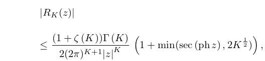
… ►Wrench (1968) gives exact values of $g_k$ up to $g_{20}$. … ►If $z$ is complex, then the remainder terms are bounded in magnitude by ${\sec }^{2n}\left(\frac{1}{2}\mathrm{ph}z\right)$ for (5.11.1), and ${\sec }^{2n+1}\left(\frac{1}{2}\mathrm{ph}z\right)$ for (5.11.2), times the first neglected terms. … ►

5.11.11 $$\left|R_K(z)\right|\le \frac{(1+\zeta \left(K\right))\mathrm{\Gamma }\left(K\right)}{2{(2\pi )}^{K+1}{\left|z\right|}^K}\left(1+\min (\sec \left(\mathrm{ph}z\right),2K^{\frac{1}{2}})\right),$$ $\left|\mathrm{ph}z\right|\le \frac{1}{2}\pi$,

ⓘ

Defines:

$R_K(z)$: remainder (locally)

Symbols:

$\mathrm{\Gamma }\left(z\right)$: gamma function, $\zeta \left(s\right)$: Riemann zeta function, $\pi$: the ratio of the circumference of a circle to its diameter, $\mathrm{ph}$: phase, $\sec z$: secant function and $z$: complex variable

Referenced by:

§5.11(ii)

Permalink:

http://dlmf.nist.gov/5.11.E11

Encodings:

pMML, png, TeX

See also:

Annotations for §5.11(ii), §5.11 and Ch.5

…

16: 4.20 Derivatives and Differential Equations

… ►

4.20.3 $$\frac{d}{dz}\tan z={\sec }^{2}z,$$

ⓘ

Symbols:

$\frac{df}{dx}$: derivative of $f$ with respect to $x$ , $\sec z$: secant function, $\tan z$: tangent function and $z$: complex variable

A&S Ref:

4.3.107

Permalink:

http://dlmf.nist.gov/4.20.E3

Encodings:

pMML, png, TeX

See also:

Annotations for §4.20 and Ch.4

… ►

4.20.5 $$\frac{d}{dz}\sec z=\sec z\tan z,$$

ⓘ

Symbols:

$\frac{df}{dx}$: derivative of $f$ with respect to $x$ , $\sec z$: secant function, $\tan z$: tangent function and $z$: complex variable

A&S Ref:

4.3.109

Permalink:

http://dlmf.nist.gov/4.20.E5

Encodings:

pMML, png, TeX

See also:

Annotations for §4.20 and Ch.4

…

17: 4.34 Derivatives and Differential Equations

… ►

4.34.3 $$\frac{d}{dz}\tanh z={\mathrm{sech}}^{2}z,$$

ⓘ

Symbols:

$\frac{df}{dx}$: derivative of $f$ with respect to $x$ , $\mathrm{sech}z$: hyperbolic secant function, $\tanh z$: hyperbolic tangent function and $z$: complex variable

A&S Ref:

4.5.73

Permalink:

http://dlmf.nist.gov/4.34.E3

Encodings:

pMML, png, TeX

See also:

Annotations for §4.34 and Ch.4

… ►

4.34.5 $$\frac{d}{dz}\mathrm{sech}z=-\mathrm{sech}z\tanh z,$$

ⓘ

Symbols:

$\frac{df}{dx}$: derivative of $f$ with respect to $x$ , $\mathrm{sech}z$: hyperbolic secant function, $\tanh z$: hyperbolic tangent function and $z$: complex variable

A&S Ref:

4.5.75

Permalink:

http://dlmf.nist.gov/4.34.E5

Encodings:

pMML, png, TeX

See also:

Annotations for §4.34 and Ch.4

…

18: 4.31 Special Values and Limits

… ►

Table 4.31.1: Hyperbolic functions: values at multiples of $\frac{1}{2}\pi \mathrm{i}$.

► ►►►

$z$	0	$\frac{1}{2}\pi \mathrm{i}$	$\pi \mathrm{i}$	$\frac{3}{2}\pi \mathrm{i}$	$\mathrm{\infty }$
…
$\mathrm{sech}z$	$1$	$\mathrm{\infty }$	$-1$	$\mathrm{\infty }$	$0$
…

►

…

19: Bibliography I

… ►

The factorization method. Rev. Modern Phys. 23 (1), pp. 21–68.

ⓘ

Referenced by:

§18.38(iii).

Encodings:

BibTeX

… ►

The real roots of Bernoulli polynomials. Ann. Univ. Turku. Ser. A I 37, pp. 1–20.

ⓘ

External Links:

MathReview (D. H. Lehmer), ZentralBlatt

Referenced by:

§24.12(i).

Encodings:

BibTeX

… ►

The $J$-matrix method. Adv. in Appl. Math. 46 (1-4), pp. 379–395.

ⓘ

External Links:

ISSN 0196-8858, Document, Link, MathReview (Boris Petrovich Osilenker)

Referenced by:

§18.39(iv).

Encodings:

BibTeX

… ►

On the asymptotic analysis of the Painlevé equations via the isomonodromy method. Nonlinearity 7 (5), pp. 1291–1325.

ⓘ

External Links:

ISSN 0951-7715, Document, MathReview (Alexander Vladimirovich Kitaev), ZentralBlatt

Referenced by:

§32.11(iii).

Encodings:

BibTeX

… ►

The Isomonodromic Deformation Method in the Theory of Painlevé Equations. Lecture Notes in Mathematics, Vol. 1191, Springer-Verlag, Berlin.

ⓘ

External Links:

ISBN 3-540-16483-9, MathReview (Alexander A. Pankov), ZentralBlatt

Referenced by:

§32.11(iv), §32.4(i), Profile Alexander A. Its.

Encodings:

BibTeX

…

20: Publications

… ►

Methods of Relevance Ranking and Hit-content Generation in Math Search, Proceedings of Mathematical Knowledge Management (MKM2007), RISC, Hagenberg, Austria, June 27–30, 2007.

►

Tensor Product B-Spline Mesh Generation for Accurate Surface Visualizations in the NIST Digital Library of Mathematical Functions, in Mathematical Methods for Curves and Surfaces, Proceedings of the 2008 International Conference on Mathematical Methods for Curves and Surfaces (MMCS 2008), Lecture Notes in Computer Science, Vol. 5862, (M. Dæhlen, M. Floater., T. Lyche, J. L. Merrien, K. Mørken, L. L. Schumaker, eds), Springer, Berlin, Heidelberg (2010) pp. 385–393.

… ►

NIST’s Digital Library of Mathematial Functions, Physics Today 71, 2, 48 (2018), pp. 48–53.