roots
(0.002 seconds)
1—10 of 83 matching pages
1: 4.46 Tables
…
►For 40D values of the first 500 roots of , see Robinson (1972).
(These roots are zeros of the Bessel function ; see §10.21.)
►For 10S values of the first five complex roots of , , and , for selected positive values of , see Fettis (1976).
…
2: 2.2 Transcendental Equations
3: 1.11 Zeros of Polynomials
…
►Roots of are , , .
…
►The square roots are chosen so that
…
►
§1.11(iv) Roots of Unity and of Other Constants
►The roots of … ►The roots of …4: 23.7 Quarter Periods
…
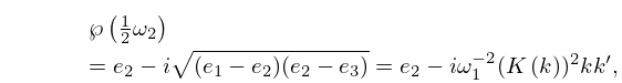
►
23.7.1
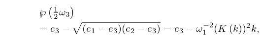
►
23.7.2
►
23.7.3
►where and the square roots are real and positive when the lattice is rectangular; otherwise they are determined by continuity from the rectangular case.
5: Tom H. Koornwinder
…
►Koornwinder has published numerous papers on special functions, harmonic analysis, Lie groups, quantum groups, computer algebra, and their interrelations, including an interpretation of Askey–Wilson polynomials on quantum SU(2), and a five-parameter extension (the Macdonald–Koornwinder polynomials) of Macdonald’s polynomials for root systems BC.
…
6: 23.21 Physical Applications
…
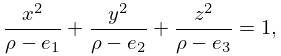
►Ellipsoidal coordinates may be defined as the three roots
of the equation
►
23.21.1
…
►
23.21.3
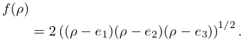
►Another form is obtained by identifying , , as lattice roots (§23.3(i)), and setting
…
7: 23.3 Differential Equations
…
►
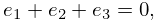
§23.3(i) Invariants, Roots, and Discriminant
… ►The lattice roots satisfy the cubic equation … ►
23.3.4
…
►
23.3.5
…
►
23.3.7
…
8: 19.38 Approximations
…
►Approximations for Legendre’s complete or incomplete integrals of all three kinds, derived by Padé approximation of the square root in the integrand, are given in Luke (1968, 1970).
…
9: 2.9 Difference Equations
…
►
2.9.4
,
►where are the roots of the characteristic equation
…
►When the roots of (2.9.5) are equal we denote them both by .
Assume first .
…
►Then the indices are the roots of
…
