relations to hyperbolic functions

SearchAdvancedHelp

(0.010 seconds)

21—30 of 45 matching pages

21: 19.1 Special Notation

… ►(For other notation see Notation for the Special Functions.) … ►The first set of main functions treated in this chapter are Legendre’s complete integrals … ►In Abramowitz and Stegun (1964, Chapter 17) the functions (19.1.1) and (19.1.2) are denoted, in order, by $K(\alpha )$, $E(\alpha )$, $\mathrm{\Pi }(n\backslash \alpha )$, $F(\varphi \backslash \alpha )$, $E(\varphi \backslash \alpha )$, and $\mathrm{\Pi }(n;\varphi \backslash \alpha )$, where $\alpha =\arcsin k$ and $n$ is the ${\alpha }^2$ (not related to $k$) in (19.1.1) and (19.1.2). … ►The second set of main functions treated in this chapter is … ►A third set of functions, introduced by Bulirsch (1965b, a, 1969a), is …

22: Bibliography F

… ►

On the reciprocal modulus relation for elliptic integrals. SIAM J. Math. Anal. 1 (4), pp. 524–526.

ⓘ

External Links:

Document, MathReview (B. C. Carlson), ZentralBlatt

Referenced by:

§19.7(i).

Encodings:

BibTeX

… ►

Numerical calculation of singular integrals related to Hankel transform. Comput. Math. Appl. 21 (2-3), pp. 87–94.

ⓘ

Notes:

Fortran, minimum precision 6D.

External Links:

ISSN 0898-1221, Document, MathReview, ZentralBlatt

Referenced by:

§10.77(ix).

Encodings:

BibTeX

… ►

Guide to tables of elliptic functions. Math. Tables and Other Aids to Computation 3 (24), pp. 229–281.

ⓘ

External Links:

FullText, MathReview (S. C. van Veen)

Referenced by:

§19.37(i).

Encodings:

BibTeX

►

Polynomial relations in the Heisenberg algebra. J. Math. Phys. 35 (11), pp. 6144–6149.

ⓘ

External Links:

ISSN 0022-2488, Document, MathReview (Shao-Ming Fei), ZentralBlatt

Referenced by:

§13.3(ii), §15.5(i), §16.3(i).

Encodings:

BibTeX

… ►

Error bounds for a uniform asymptotic expansion of the Legendre function $Q_n^{-m}(\cosh z)$ . SIAM J. Math. Anal. 21 (2), pp. 523–535.

ⓘ

External Links:

ISSN 0036-1410, Document, MathReview (F. W. J. Olver), ZentralBlatt

Referenced by:

§14.26.

Encodings:

BibTeX

…

23: 6.2 Definitions and Interrelations

… ►This is also true of the functions $\mathrm{Ci}\left(z\right)$ and $\mathrm{Chi}\left(z\right)$ defined in §6.2(ii). … ►The logarithmic integral is defined by … ► $\mathrm{Si}\left(z\right)$ is an odd entire function. … ►

Hyperbolic Analogs of the Sine and Cosine Integrals

… ►

§6.2(iii) Auxiliary Functions

…

24: 18.28 Askey–Wilson Class

… ►

§18.28(ii) Askey–Wilson Polynomials

… ►

Recurrence Relation

… ►

§18.28(viii) $q$-Racah Polynomials

… ►

§18.28(x) Limit Relations

… ►Genest et al. (2016) showed that these polynomials coincide with the nonsymmetric Wilson polynomials in Groenevelt (2007).

25: 19.25 Relations to Other Functions

§19.25 Relations to Other Functions

… ►

§19.25(iv) Theta Functions

… ► … ►

§19.25(vii) Hypergeometric Function

… ►

26: 27.14 Unrestricted Partitions

… ►where $p\left(k\right)$ is defined to be $0$ if . … ►These recursions can be used to calculate $p\left(n\right)$, which grows very rapidly. … ►

§27.14(iv) Relation to Modular Functions

… ►This is related to the function $f\left(x\right)$ in (27.14.2) by … ►The tau function is multiplicative and satisfies the more general relation: …

27: Bibliography B

… ►

Orthogonality relations for the associated Legendre functions of imaginary order. Integral Transforms Spec. Funct. 24 (4), pp. 331–337.

ⓘ

External Links:

ISSN 1065-2469, Document, FullText, MathReview (Praveen Agarwal), ZentralBlatt

Referenced by:

§14.17(iii), §14.17(iii).

Encodings:

BibTeX

… ►

Tables Relating to the Radial Mathieu Functions. Vol. 1: Functions of the First Kind. U.S. Government Printing Office, Washington, D.C..

ⓘ

External Links:

MathReview (C. J. Bouwkamp)

Referenced by:

1st item.

Encodings:

BibTeX

►

Tables Relating to the Radial Mathieu Functions. Vol. 2: Functions of the Second Kind. U.S. Government Printing Office, Washington, D.C..

ⓘ

External Links:

MathReview (C. J. Bouwkamp)

Referenced by:

2nd item, 1st item.

Encodings:

BibTeX

… ►

Bessel functions and modular relations of higher type and hyperbolic differential equations. Comm. Sém. Math. Univ. Lund [Medd. Lunds Univ. Mat. Sem.] 1952 (Tome Supplementaire), pp. 12–20.

ⓘ

External Links:

MathReview (S. C. van Veen), ZentralBlatt

Referenced by:

§35.5(i).

Encodings:

BibTeX

… ►

Concerning the zeros of some functions related to Bessel functions. J. Mathematical Phys. 10 (9), pp. 1729–1744.

ⓘ

External Links:

Document, MathReview (C. V. Coffman), ZentralBlatt

Referenced by:

§10.21(xi).

Encodings:

BibTeX

…

28: 19.2 Definitions

… ►Also, if $k^2$ and ${\alpha }^2$ are real, then $\mathrm{\Pi }(\varphi ,{\alpha }^2,k)$ is called a circular or hyperbolic case according as ${\alpha }^2({\alpha }^2-k^2)({\alpha }^2-1)$ is negative or positive. … ►

§19.2(iv) A Related Function: $R_C(x,y)$

… ►In (19.2.18)–(19.2.22) the inverse trigonometric and hyperbolic functions assume their principal values (§§4.23(ii) and 4.37(ii)). When $x$ and $y$ are positive, $R_C(x,y)$ is an inverse circular function if and an inverse hyperbolic function (or logarithm) if $x>y$: …The Cauchy principal value is hyperbolic: …

29: 14.3 Definitions and Hypergeometric Representations

§14.3 Definitions and Hypergeometric Representations

►

§14.3(i) Interval

… ►

§14.3(ii) Interval

… ►

§14.3(iii) Alternative Hypergeometric Representations

… ►

§14.3(iv) Relations to Other Functions

…

30: Errata

… ►

The Gegenbauer function $C_{\alpha }^{(\lambda )}\left(z\right)$, was labeled inadvertently as the ultraspherical (Gegenbauer) polynomial $C_n^{(\lambda )}\left(z\right)$. In order to resolve this inconsistency, this function now links correctly to its definition. This change affects Gegenbauer functions which appear in §§14.3(iv), 15.9(iii).

… ►

Scales were corrected in all figures. The interval $-8.4\le \frac{x-y}{\sqrt{2}}\le 8.4$ was replaced by $-12.0\le \frac{x-y}{\sqrt{2}}\le 12.0$ and $-12.7\le \frac{x+y}{\sqrt{2}}\le 4.2$ replaced by $-18.0\le \frac{x+y}{\sqrt{2}}\le 6.0$. All plots and interactive visualizations were regenerated to improve image quality.

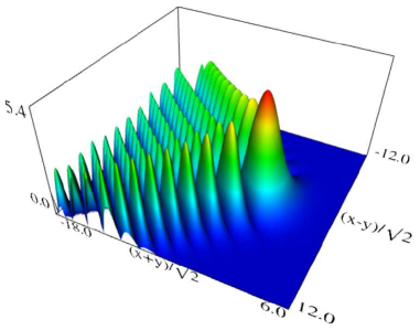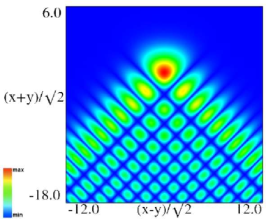
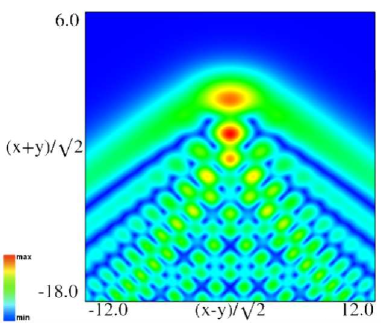
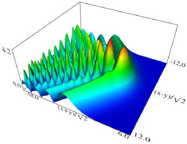
(a) Density plot.	(b) 3D plot.

Figure 36.3.9: Modulus of hyperbolic umbilic canonical integral function $|{\mathrm{\Psi }}^{(\mathrm{H})}\left(x,y,0\right)|$.

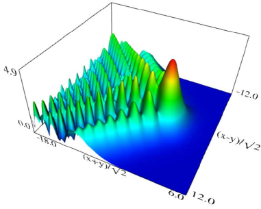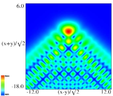
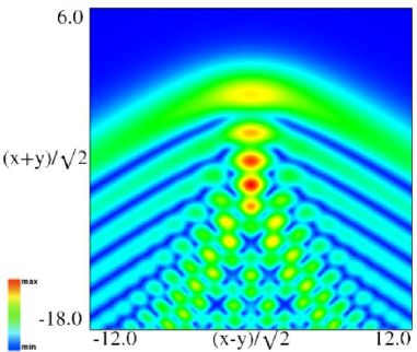
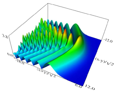
(a) Density plot.	(b) 3D plot.

Figure 36.3.10: Modulus of hyperbolic umbilic canonical integral function $|{\mathrm{\Psi }}^{(\mathrm{H})}\left(x,y,1\right)|$.

(a) Density plot.	(b) 3D plot.

Figure 36.3.11: Modulus of hyperbolic umbilic canonical integral function $|{\mathrm{\Psi }}^{(\mathrm{H})}\left(x,y,2\right)|$.

(a) Density plot.	(b) 3D plot.

Figure 36.3.12: Modulus of hyperbolic umbilic canonical integral function $|{\mathrm{\Psi }}^{(\mathrm{H})}\left(x,y,3\right)|$.

Reported 2016-09-12 by Dan Piponi.

►

The scaling error reported on 2016-09-12 by Dan Piponi also applied to contour and density plots for the phase of the hyperbolic umbilic canonical integrals. Scales were corrected in all figures. The interval $-8.4\le \frac{x-y}{\sqrt{2}}\le 8.4$ was replaced by $-12.0\le \frac{x-y}{\sqrt{2}}\le 12.0$ and $-12.7\le \frac{x+y}{\sqrt{2}}\le 4.2$ replaced by $-18.0\le \frac{x+y}{\sqrt{2}}\le 6.0$. All plots and interactive visualizations were regenerated to improve image quality.

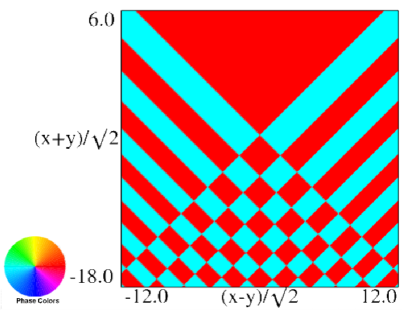(a) Contour plot.	(b) Density plot.

Figure 36.3.18: Phase of hyperbolic umbilic canonical integral $\mathrm{ph}{\mathrm{\Psi }}^{(\mathrm{H})}\left(x,y,0\right)$.

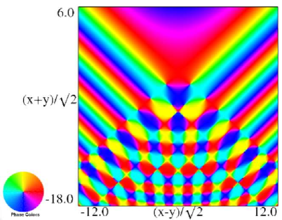(a) Contour plot.	(b) Density plot.

Figure 36.3.19: Phase of hyperbolic umbilic canonical integral $\mathrm{ph}{\mathrm{\Psi }}^{(\mathrm{H})}\left(x,y,1\right)$.

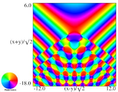(a) Contour plot.	(b) Density plot.

Figure 36.3.20: Phase of hyperbolic umbilic canonical integral $\mathrm{ph}{\mathrm{\Psi }}^{(\mathrm{H})}\left(x,y,2\right)$.

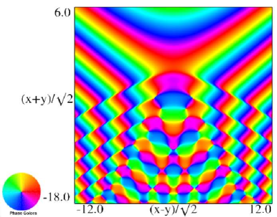(a) Contour plot.	(b) Density plot.

Figure 36.3.21: Phase of hyperbolic umbilic canonical integral $\mathrm{ph}{\mathrm{\Psi }}^{(\mathrm{H})}\left(x,y,3\right)$.

Reported 2016-09-28.

… ►

A number of additions and changes have been made to the metadata to reflect new and changed references as well as to how some equations have been derived.

… ►

Originally the limiting form for $\mathrm{sc}(z,k)$ in the last line of this table was incorrect ($\cosh z$, instead of $\sinh z$).

$\mathrm{sn}(z,k)$ $\to$	$\tanh z$	$\mathrm{cd}(z,k)$ $\to$	$1$	$\mathrm{dc}(z,k)$ $\to$	$1$	$\mathrm{ns}(z,k)$ $\to$	$\coth z$
$\mathrm{cn}(z,k)$ $\to$	$\mathrm{sech}z$	$\mathrm{sd}(z,k)$ $\to$	$\sinh z$	$\mathrm{nc}(z,k)$ $\to$	$\cosh z$	$\mathrm{ds}(z,k)$ $\to$	$\mathrm{csch}z$
$\mathrm{dn}(z,k)$ $\to$	$\mathrm{sech}z$	$\mathrm{nd}(z,k)$ $\to$	$\cosh z$	$\mathrm{sc}(z,k)$ $\to$	$\sinh z$	$\mathrm{cs}(z,k)$ $\to$	$\mathrm{csch}z$

Reported 2010-11-23.

…