q-multinomial%20coefficient
(0.002 seconds)
21—30 of 293 matching pages
21: 12.10 Uniform Asymptotic Expansions for Large Parameter
…
►The coefficients are given by
…
►and the coefficients
are defined by
…
►and the coefficients
and are given by
…
►The coefficients
and are given by
…The coefficients
and in (12.10.36) and (12.10.38) are given by
…
22: 3.8 Nonlinear Equations
…
►However, when the coefficients are all real, complex arithmetic can be avoided by the following iterative process.
…
►Thus if is the polynomial (3.8.8) and is the coefficient
, say, then
…
►
3.8.15
…
►Consider and .
We have and .
…
23: 36 Integrals with Coalescing Saddles
…
24: Gergő Nemes
…
►As of September 20, 2021, Nemes performed a complete analysis and acted as main consultant for the update of the source citation and proof metadata for every formula in Chapter 25 Zeta and Related Functions.
…
25: Wolter Groenevelt
…
►As of September 20, 2022, Groenevelt performed a complete analysis and acted as main consultant for the update of the source citation and proof metadata for every formula in Chapter 18 Orthogonal Polynomials.
…
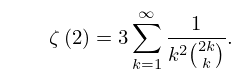
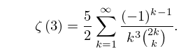
26: 25.6 Integer Arguments
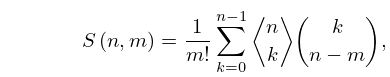
27: 26.14 Permutations: Order Notation
28: 33.24 Tables
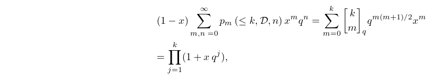
29: 26.10 Integer Partitions: Other Restrictions
…
►
Table 26.10.1: Partitions restricted by difference conditions, or equivalently with parts from .
►
►
►
…
►
| … | ||||
26.10.3
,
…
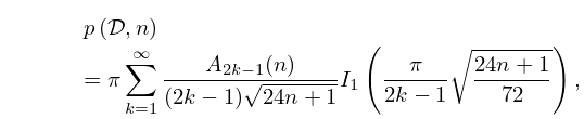
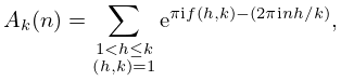
►
26.10.17
►where is the modified Bessel function (§10.25(ii)), and
►
26.10.18
…
