open disks around infinity
(0.002 seconds)
11—20 of 534 matching pages
11: 18.40 Methods of Computation
…
►Let .
…
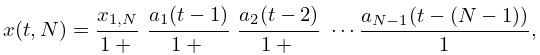
►Here is an interpolation of the abscissas , that is, , allowing differentiation by .
…
►
18.40.9
,
…
►The PWCF is a minimally oscillatory algebraic interpolation of the abscissas .
…
►Further, exponential convergence in , via the Derivative Rule, rather than the power-law convergence of the histogram methods, is found for the inversion of Gegenbauer, Attractive, as well as Repulsive, Coulomb–Pollaczek, and Hermite weights and zeros to approximate for these OP systems on and respectively, Reinhardt (2018), and Reinhardt (2021b), Reinhardt (2021a).
…
12: 28.17 Stability as
§28.17 Stability as
►If all solutions of (28.2.1) are bounded when along the real axis, then the corresponding pair of parameters is called stable. … ►However, if , then always comprises an unstable pair. For example, as one of the solutions and tends to and the other is unbounded (compare Figure 28.13.5). … ►For real and the stable regions are the open regions indicated in color in Figure 28.17.1. …13: 1.4 Calculus of One Variable
…
►If is continuous at each point , then is continuous on the interval
and we write .
…
►If exists and is continuous on an interval , then we write .
…
►Then for continuous on ,
…
►If , then is of bounded
variation on .
…
►A function is convex on if
…
14: 18.1 Notation
15: 31.4 Solutions Analytic at Two Singularities: Heun Functions
…
►For an infinite set of discrete values , , of the accessory parameter , the function is analytic at , and hence also throughout the disk
.
…
►with , denotes a set of solutions of (31.2.1), each of which is analytic at and .
…
16: 4.23 Inverse Trigonometric Functions
…
►The function assumes its principal value when ; elsewhere on the integration paths the branch is determined by continuity.
…
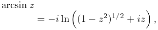
►
4.23.19
;
…
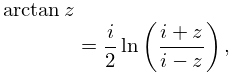
►
4.23.26
;
…
►Care needs to be taken on the cuts, for example, if then .
…
►where and in (4.23.34) and (4.23.35), and in (4.23.36).
…
17: 18.3 Definitions
…
►
2.
…
►
Table 18.3.1: Orthogonality properties for classical OP’s: intervals, weight functions, standardizations, leading coefficients, and parameter constraints.
…
►
►
►
…
►For a finite system of Jacobi polynomials is orthogonal on with weight function .
For and a finite system of Jacobi polynomials (called pseudo Jacobi polynomials or Routh–Romanovski polynomials) is orthogonal on with .
…
With the property that is again a system of OP’s. See §18.9(iii).
| Name | Constraints | ||||||
|---|---|---|---|---|---|---|---|
| … | |||||||
| Hermite | |||||||
| Hermite | |||||||
18: 7.24 Approximations
…
►
•
►
•
…
Schonfelder (1978) gives coefficients of Chebyshev expansions for on , for on , and for on (30D).
Shepherd and Laframboise (1981) gives coefficients of Chebyshev series for on (22D).
19: 23.20 Mathematical Applications
…
►Points on the curve can be parametrized by , , where and : in this case we write .
The curve is made into an abelian group (Macdonald (1968, Chapter 5)) by defining the zero element as the point at infinity, the negative of by , and generally on the curve iff the points , , are collinear.
…
►In terms of the addition law can be expressed , ; otherwise , where
…
►
always has the form (Mordell’s Theorem: Silverman and Tate (1992, Chapter 3, §5)); the determination of , the rank of , raises questions of great difficulty, many of which are still open.
…To determine , we make use of the fact that if then must be a divisor of ; hence there are only a finite number of possibilities for .
…
20: 14.21 Definitions and Basic Properties
…
►
and exist for all values of , , and , except possibly and , which are branch points (or poles) of the functions, in general.
When is complex , , and are defined by (14.3.6)–(14.3.10) with replaced by : the principal branches are obtained by taking the principal values of all the multivalued functions appearing in these representations when , and by continuity elsewhere in the -plane with a cut along the interval ; compare §4.2(i).
The principal branches of and are real when , and .
…
►Many of the properties stated in preceding sections extend immediately from the -interval to the cut -plane .
…
