open
(0.001 seconds)
21—30 of 195 matching pages
21: 14.21 Definitions and Basic Properties
…
►When is complex , , and are defined by (14.3.6)–(14.3.10) with replaced by : the principal branches are obtained by taking the principal values of all the multivalued functions appearing in these representations when , and by continuity elsewhere in the -plane with a cut along the interval ; compare §4.2(i).
The principal branches of and are real when , and .
…
►Many of the properties stated in preceding sections extend immediately from the -interval to the cut -plane .
…
22: 18.16 Zeros
…
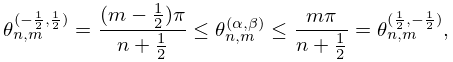
►Let , , denote the zeros of as function of with
…
►
18.16.2
,
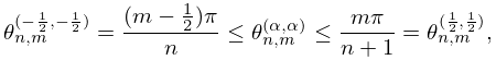
►
18.16.3
,
.
…
►when .
…
►All zeros of lie in the open interval .
…
23: 23.15 Definitions
…
►The set of all bilinear transformations of this form is denoted by SL (Serre (1973, p. 77)).
►A modular function
is a function of that is meromorphic in the half-plane , and has the property that for all , or for all belonging to a subgroup of SL,
…
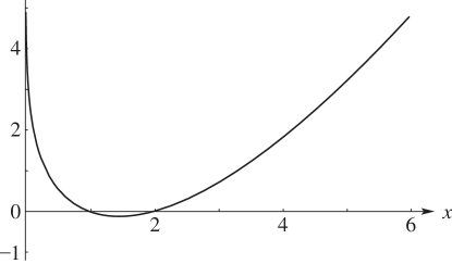
24: 8.13 Zeros
25: 1.6 Vectors and Vector-Valued Functions
…
►Note: The terminology open and closed sets and boundary
points in the plane that is used in this subsection and §1.6(v) is analogous to that introduced for the complex plane in §1.9(ii).
…
►and be the closed and bounded point set in the plane having a simple closed curve as boundary.
…
►with , an open set in the plane.
…
►The vector at is normal to the surface at .
…
26: 22.18 Mathematical Applications
…
►The half-open rectangle maps onto cut along the intervals and .
…
►For any two points and on this curve, their sum
, always a third point on the curve, is defined by the Jacobi–Abel addition law
…
27: 26.9 Integer Partitions: Restricted Number and Part Size
…
►It is also equal to the number of lattice paths from to that have exactly vertices , , , above and to the left of the lattice path.
…
28: 5.3 Graphics
29: 18.2 General Orthogonal Polynomials
…
►Let be a finite or infinite open interval in .
…
►Assume in (18.2.12).
…
►(convergence in ).
…
►This is the class of weight functions on such that, in addition to (18.2.1_5),
…
►
