of arbitrary order
(0.002 seconds)
41—49 of 49 matching pages
41: 13.2 Definitions and Basic Properties
…
►where is an arbitrary small positive constant.
…
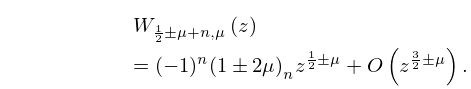
►
13.2.13
…
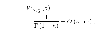
►
13.2.14
…
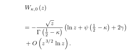
►
13.2.16
, ,
…
►where is an arbitrary small positive constant.
…
42: Bibliography
…
►
Polygamma functions of negative order.
J. Comput. Appl. Math. 100 (2), pp. 191–199.
…
►
On the degrees of irreducible factors of higher order Bernoulli polynomials.
Acta Arith. 62 (4), pp. 329–342.
►
Congruences of -adic integer order Bernoulli numbers.
J. Number Theory 59 (2), pp. 374–388.
…
►
Algorithm 804: Subroutines for the computation of Mathieu functions of integer orders.
ACM Trans. Math. Software 26 (3), pp. 408–414.
…
►
A subroutine package for Bessel functions of a complex argument and nonnegative order.
Technical Report
Technical Report SAND85-1018, Sandia National Laboratories, Albuquerque, NM.
…
43: 15.12 Asymptotic Approximations
…
►Let denote an arbitrary small positive constant.
…
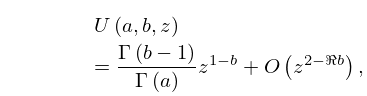
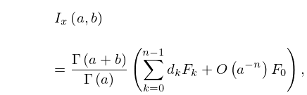
►
15.12.2
.
…
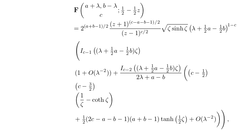
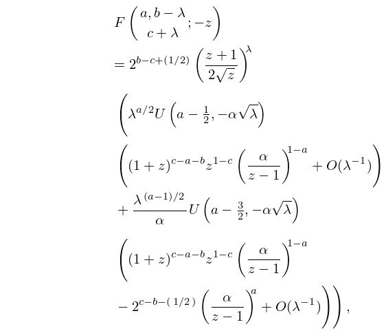
►Again, throughout this subsection denotes an arbitrary small positive constant, and are real or complex and fixed.
…
►
15.12.5
…
►
15.12.7
…
44: 2.8 Differential Equations with a Parameter
…
►For example, can be the order of a Bessel function or degree of an orthogonal polynomial.
…
►(the constants of integration being arbitrary).
…
►
§2.8(iv) Case III: Simple Pole
… ►For a coalescing turning point and double pole see Boyd and Dunster (1986) and Dunster (1990b); in this case the uniform approximants are Bessel functions of variable order. … ►Lastly, for an example of a fourth-order differential equation, see Wong and Zhang (2007). …45: 15.11 Riemann’s Differential Equation
…
►The importance of (15.10.1) is that any homogeneous linear differential equation of the second order with at most three distinct singularities, all regular, in the extended plane can be transformed into (15.10.1).
…
►The reduction of a general homogeneous linear differential equation of the second order with at most three regular singularities to the hypergeometric differential equation is given by
…
►for arbitrary
and .
46: 13.14 Definitions and Basic Properties
…
►
13.14.14
.
…
►
13.14.15
…
►
13.14.17
…
►
13.14.19
…
►where is an arbitrary small positive constant.
…
47: 18.39 Applications in the Physical Sciences
…
►The nature of, and notations and common vocabulary for, the eigenvalues and eigenfunctions of self-adjoint second order differential operators is overviewed in §1.18.
…
►The fundamental quantum Schrödinger operator, also called the Hamiltonian, , is a second order differential operator of the form
…
►
is referred to as the ground state, all others, in order of increasing energy being excited states.
…
►If is an arbitrary unit normalized function in the domain of then, by self-adjointness,
…
►(where the minus sign is often omitted, as it arises as an arbitrary phase when taking the square root of the real, positive, norm of the wave function), allowing equation (18.39.37) to be rewritten in terms of the associated Coulomb–Laguerre polynomials .
…
48: 8.18 Asymptotic Expansions of
…
►
8.18.1
…
►
8.18.3
…
►uniformly for and , , where again denotes an arbitrary small positive constant.
…
49: 3.8 Nonlinear Equations
…
►for all sufficiently large, where and are independent of , then the sequence is said to have convergence of the
th order.
…
…
►This is useful when satisfies a second-order linear differential equation because of the ease of computing .
…
►For describing the distribution of complex zeros of solutions of linear homogeneous second-order differential equations by methods based on the Liouville–Green (WKB) approximation, see Segura (2013).
…
►For an arbitrary starting point , convergence cannot be predicted, and the boundary of the set of points that generate a sequence converging to a particular zero has a very complicated structure.
…
