metric coefficients
(0.009 seconds)
11—20 of 241 matching pages
11: 29.21 Tables
…
►
•
Arscott and Khabaza (1962) tabulates the coefficients of the polynomials in Table 29.12.1 (normalized so that the numerically largest coefficient is unity, i.e. monic polynomials), and the corresponding eigenvalues for , . Equations from §29.6 can be used to transform to the normalization adopted in this chapter. Precision is 6S.
12: 34.1 Special Notation
…
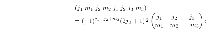
►An often used alternative to the symbol is the Clebsch–Gordan coefficient
►
34.1.1
…
►For other notations for , , symbols, see Edmonds (1974, pp. 52, 97, 104–105) and Varshalovich et al. (1988, §§8.11, 9.10, 10.10).
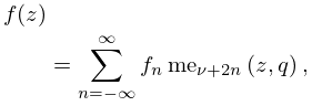
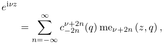
13: 28.19 Expansions in Series of Functions
14: 26.16 Multiset Permutations
…
►The number of elements in is the multinomial coefficient (§26.4) .
…
►Thus , and
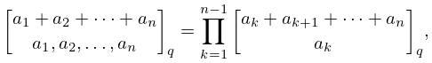
►The
-multinomial coefficient is defined in terms of Gaussian polynomials (§26.9(ii)) by
►
26.16.1
…
►
26.16.2
…
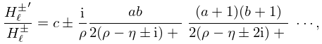
15: 33.8 Continued Fractions
…
►
33.8.2
…
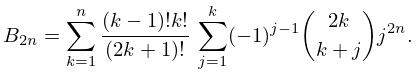
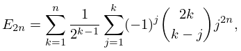
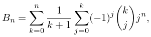
16: 24.6 Explicit Formulas
17: 20.6 Power Series
18: 2.9 Difference Equations
…
►Often and can be expanded in series
…Formal solutions are
…
►
, and higher coefficients are determined by formal substitution.
…
►with and higher coefficients given by (2.9.7) (in the present case the coefficients of and are zero).
…
►The coefficients
and constant are again determined by formal substitution, beginning with when , or with when .
…
19: 16.24 Physical Applications
…
►
