machine epsilon

SearchAdvancedHelp

(0.001 seconds)

1—10 of 69 matching pages

1: 22.16 Related Functions

… ►

§22.16(ii) Jacobi’s Epsilon Function

►

Integral Representations

… ►See Figure 22.16.2. … ►

Quasi-Addition and Quasi-Periodic Formulas

… ►

Relation to Theta Functions

…

2: 3.1 Arithmetics and Error Measures

… ► … ► … ►The machine epsilon ${ϵ}_M$, that is, the distance between $1$ and the next larger machine number with $E=0$ is given by ${ϵ}_M=2^{-p+1}$. The machine precision is $\frac{1}{2}{ϵ}_M=2^{-p}$. … ►Symmetric rounding or rounding to nearest of $x$ gives $x_{-}$ or $x_{+}$, whichever is nearer to $x$, with maximum relative error equal to the machine precision $\frac{1}{2}{ϵ}_M=2^{-p}$. …

3: 27.15 Chinese Remainder Theorem

… ►Even though the lengthy calculation is repeated four times, once for each modulus, most of it only uses five-digit integers and is accomplished quickly without overwhelming the machine’s memory. Details of a machine program describing the method together with typical numerical results can be found in Newman (1967). …

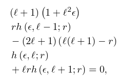
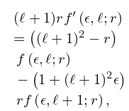
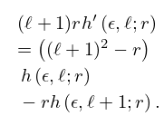
4: 33.17 Recurrence Relations and Derivatives

§33.17 Recurrence Relations and Derivatives

►

33.17.1 $$(\mathrm{\ell }+1)rf(ϵ,\mathrm{\ell }-1;r)-(2\mathrm{\ell }+1)\left(\mathrm{\ell }(\mathrm{\ell }+1)-r\right)f(ϵ,\mathrm{\ell };r)+\mathrm{\ell }\left(1+{(\mathrm{\ell }+1)}^2ϵ\right)rf(ϵ,\mathrm{\ell }+1;r)=0,$$

ⓘ

Symbols:

$f(ϵ,\mathrm{\ell };r)$: regular Coulomb function, $\mathrm{\ell }$: nonnegative integer, $r$: real variable and $ϵ$: real parameter

Permalink:

http://dlmf.nist.gov/33.17.E1

Encodings:

pMML, png, TeX

See also:

Annotations for §33.17 and Ch.33

►

33.17.2 $$(\mathrm{\ell }+1)\left(1+{\mathrm{\ell }}^2ϵ\right)rh(ϵ,\mathrm{\ell }-1;r)-(2\mathrm{\ell }+1)\left(\mathrm{\ell }(\mathrm{\ell }+1)-r\right)h(ϵ,\mathrm{\ell };r)+\mathrm{\ell }rh(ϵ,\mathrm{\ell }+1;r)=0,$$

ⓘ

Symbols:

$h(ϵ,\mathrm{\ell };r)$: irregular Coulomb function, $\mathrm{\ell }$: nonnegative integer, $r$: real variable and $ϵ$: real parameter

Permalink:

http://dlmf.nist.gov/33.17.E2

Encodings:

pMML, png, TeX

See also:

Annotations for §33.17 and Ch.33

►

33.17.3 $$(\mathrm{\ell }+1)r{f}^{\prime }(ϵ,\mathrm{\ell };r)=\left({(\mathrm{\ell }+1)}^2-r\right)f(ϵ,\mathrm{\ell };r)-\left(1+{(\mathrm{\ell }+1)}^2ϵ\right)rf(ϵ,\mathrm{\ell }+1;r),$$

ⓘ

Symbols:

$f(ϵ,\mathrm{\ell };r)$: regular Coulomb function, $\mathrm{\ell }$: nonnegative integer, $r$: real variable and $ϵ$: real parameter

Permalink:

http://dlmf.nist.gov/33.17.E3

Encodings:

pMML, png, TeX

See also:

Annotations for §33.17 and Ch.33

►

33.17.4 $$(\mathrm{\ell }+1)r{h}^{\prime }(ϵ,\mathrm{\ell };r)=\left({(\mathrm{\ell }+1)}^2-r\right)h(ϵ,\mathrm{\ell };r)-rh(ϵ,\mathrm{\ell }+1;r).$$

ⓘ

Symbols:

$h(ϵ,\mathrm{\ell };r)$: irregular Coulomb function, $\mathrm{\ell }$: nonnegative integer, $r$: real variable and $ϵ$: real parameter

Permalink:

http://dlmf.nist.gov/33.17.E4

Encodings:

pMML, png, TeX

See also:

Annotations for §33.17 and Ch.33

5: 33.15 Graphics

§33.15 Graphics

►

§33.15(i) Line Graphs of the Coulomb Functions $f(ϵ,\mathrm{\ell };r)$ and $h(ϵ,\mathrm{\ell };r)$

►

►►

Figure 33.15.1: $f(ϵ,\mathrm{\ell };r),h(ϵ,\mathrm{\ell };r)$ with $\mathrm{\ell }=0,ϵ=4$. Magnify

… ►

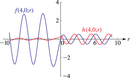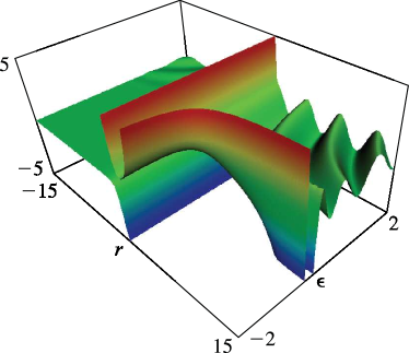
§33.15(ii) Surfaces of the Coulomb Functions $f(ϵ,\mathrm{\ell };r)$, $h(ϵ,\mathrm{\ell };r)$, $s(ϵ,\mathrm{\ell };r)$, and $c(ϵ,\mathrm{\ell };r)$

… ►

►

►

Figure 33.15.9: $h(ϵ,\mathrm{\ell };r)$ with . Magnify 3D Help

…

6: 33.14 Definitions and Basic Properties

… ►This includes $ϵ=0$, hence $f(ϵ,\mathrm{\ell };r)$ can be expanded in a convergent power series in $ϵ$ in a neighborhood of $ϵ=0$ (§33.20(ii)). … ►

§33.14(iv) Solutions $s(ϵ,\mathrm{\ell };r)$ and $c(ϵ,\mathrm{\ell };r)$

… ►An alternative formula for $A(ϵ,\mathrm{\ell })$ is … ►

§33.14(v) Wronskians

►With arguments $ϵ,\mathrm{\ell },r$ suppressed, …

7: 33.1 Special Notation

… ► ►►►

$k,\mathrm{\ell }$	nonnegative integers.
…
$ϵ,\eta$	real parameters.
…

►The main functions treated in this chapter are first the Coulomb radial functions $F_{\mathrm{\ell }}(\eta ,\rho )$, $G_{\mathrm{\ell }}(\eta ,\rho )$, $H_{\mathrm{\ell }}^{\pm }(\eta ,\rho )$ (Sommerfeld (1928)), which are used in the case of repulsive Coulomb interactions, and secondly the functions $f(ϵ,\mathrm{\ell };r)$, $h(ϵ,\mathrm{\ell };r)$, $s(ϵ,\mathrm{\ell };r)$, $c(ϵ,\mathrm{\ell };r)$ (Seaton (1982, 2002a)), which are used in the case of attractive Coulomb interactions. … ►

$P_{\mathrm{\ell }}(ϵ,r)=(2\mathrm{\ell }+1)!f(ϵ,\mathrm{\ell };r)/2^{\mathrm{\ell }+1}$, $Q_{\mathrm{\ell }}(ϵ,r)=-(2\mathrm{\ell }+1)!h(ϵ,\mathrm{\ell };r)/(2^{\mathrm{\ell }+1}A(ϵ,\mathrm{\ell }))$.

►

$f^{(0)}(ϵ,\mathrm{\ell };r)=f(ϵ,\mathrm{\ell };r)$, $f(ϵ,\mathrm{\ell };r)=s(ϵ,\mathrm{\ell };r)$, $g(ϵ,\mathrm{\ell };r)=c(ϵ,\mathrm{\ell };r)$.

8: 33.18 Limiting Forms for Large $\mathrm{\ell }$

§33.18 Limiting Forms for Large $\mathrm{\ell }$

►As $\mathrm{\ell }\to \mathrm{\infty }$ with $ϵ$ and $r$ ($\ne 0$) fixed, ►

$f(ϵ,\mathrm{\ell };r)\sim {\displaystyle \frac{{(2r)}^{\mathrm{\ell }+1}}{(2\mathrm{\ell }+1)!}},$

►

$h(ϵ,\mathrm{\ell };r)\sim {\displaystyle \frac{(2\mathrm{\ell })!}{\pi {(2r)}^{\mathrm{\ell }}}}.$

9: 33.24 Tables

§33.24 Tables

… ►

Curtis (1964a) tabulates $P_{\mathrm{\ell }}(ϵ,r)$, $Q_{\mathrm{\ell }}(ϵ,r)$ (§33.1), and related functions for $\mathrm{\ell }=0,1,2$ and $ϵ=-2(.2)2$, with $x=0(.1)4$ for and $x=0(.1)10$ for $ϵ\ge 0$; 6D.

…

10: 33.20 Expansions for Small $|ϵ|$

… ►

§33.20(i) Case $ϵ=0$

… ►

§33.20(ii) Power-Series in $ϵ$ for the Regular Solution

… ►The series (33.20.3) converges for all $r$ and $ϵ$. ►

§33.20(iii) Asymptotic Expansion for the Irregular Solution

… ►

§33.20(iv) Uniform Asymptotic Expansions

…