limiting forms as order tends to integers

SearchAdvancedHelp

(0.007 seconds)

1—10 of 929 matching pages

1: 1.13 Differential Equations

… ►

§1.13(vii) Closed-Form Solutions

… ►

§1.13(viii) Eigenvalues and Eigenfunctions: Sturm-Liouville and Liouville forms

… ►This is the Sturm-Liouville form of a second order differential equation, where ^′ denotes $\frac{d}{dx}$. … ►

Transformation to Liouville normal Form

►Equation (1.13.26) with $x\in [a,b]$ may be transformed to the Liouville normal form …

2: 28.2 Definitions and Basic Properties

… ►The standard form of Mathieu’s equation with parameters $(a,q)$ is …With $\zeta ={\sin }^{2}z$ we obtain the algebraic form of Mathieu’s equation …With $\zeta =\cos z$ we obtain another algebraic form: … ►leads to a Floquet solution. … ►

§28.2(vi) Eigenfunctions

…

3: 28.12 Definitions and Basic Properties

… ►

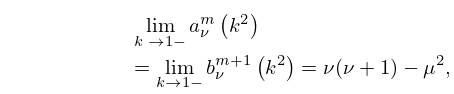
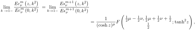
§28.12(ii) Eigenfunctions ${\mathrm{me}}_{\nu }(z,q)$

… ►However, these functions are not the limiting values of ${\mathrm{me}}_{\pm \nu }(z,q)$ as $\nu \to n$ $(\ne 0)$. … ►Again, the limiting values of ${\mathrm{ce}}_{\nu }(z,q)$ and ${\mathrm{se}}_{\nu }(z,q)$ as $\nu \to n$ $(\ne 0)$ are not the functions ${\mathrm{ce}}_n(z,q)$ and ${\mathrm{se}}_n(z,q)$ defined in §28.2(vi). …

4: 33.18 Limiting Forms for Large $\mathrm{\ell }$

§33.18 Limiting Forms for Large $\mathrm{\ell }$

►As $\mathrm{\ell }\to \mathrm{\infty }$ with $ϵ$ and $r$ ($\ne 0$) fixed, …

5: 10.24 Functions of Imaginary Order

§10.24 Functions of Imaginary Order

… ►and ${\tilde{J}}_{\nu }\left(x\right)$, ${\tilde{Y}}_{\nu }\left(x\right)$ are linearly independent solutions of (10.24.1): … ►In consequence of (10.24.6), when $x$ is large ${\tilde{J}}_{\nu }\left(x\right)$ and ${\tilde{Y}}_{\nu }\left(x\right)$ comprise a numerically satisfactory pair of solutions of (10.24.1); compare §2.7(iv). … … ►

6: 10.45 Functions of Imaginary Order

§10.45 Functions of Imaginary Order

… ►and ${\tilde{I}}_{\nu }\left(x\right)$, ${\tilde{K}}_{\nu }\left(x\right)$ are real and linearly independent solutions of (10.45.1): … ►The corresponding result for ${\tilde{K}}_{\nu }\left(x\right)$ is given by … ► … ►

7: 26.3 Lattice Paths: Binomial Coefficients

… ►

§26.3(i) Definitions

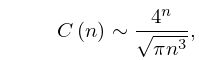
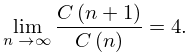
► $\left(\genfrac{}{}{0.0pt}{}{m}{n}\right)$ is the number of ways of choosing $n$ objects from a collection of $m$ distinct objects without regard to order. $\left(\genfrac{}{}{0.0pt}{}{m+n}{n}\right)$ is the number of lattice paths from $(0,0)$ to $(m,n)$. …The number of lattice paths from $(0,0)$ to $(m,n)$, $m\le n$, that stay on or above the line $y=x$ is $\left(\genfrac{}{}{0.0pt}{}{m+n}{m}\right)-\left(\genfrac{}{}{0.0pt}{}{m+n}{m-1}\right).$ … ►

§26.3(v) Limiting Form

…

8: 34.8 Approximations for Large Parameters

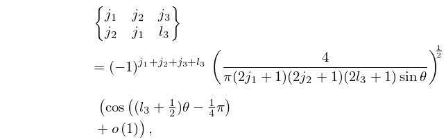
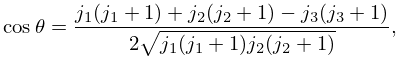
… ►For large values of the parameters in the $\mathit{3}j$, $\mathit{6}j$, and $\mathit{9}j$ symbols, different asymptotic forms are obtained depending on which parameters are large. … ►

34.8.1 $j_1,j_2,j_3\gg l_3\gg 1$,

ⓘ

Symbols:

$\pi$: the ratio of the circumference of a circle to its diameter, $\cos z$: cosine function, $o\left(x\right)$: order less than, $\sin z$: sine function, : $\mathit{6}j$ symbol, $j,j_r$: non-negative integers or non-negative integers plus one half. and $l,l_r$: non-negative integers or non-negative integers plus one half.

Permalink:

http://dlmf.nist.gov/34.8.E1

Encodings:

pMML, png, TeX

See also:

Annotations for §34.8 and Ch.34

… ►

34.8.2 $$\cos \theta =\frac{j_1(j_1+1)+j_2(j_2+1)-j_3(j_3+1)}{2\sqrt{j_1(j_1+1)j_2(j_2+1)}},$$

ⓘ

Symbols:

$\cos z$: cosine function and $j,j_r$: non-negative integers or non-negative integers plus one half.

Permalink:

http://dlmf.nist.gov/34.8.E2

Encodings:

pMML, png, TeX

See also:

Annotations for §34.8 and Ch.34

►and the symbol $o\left(1\right)$ denotes a quantity that tends to zero as the parameters tend to infinity, as in §2.1(i). …

9: 29.5 Special Cases and Limiting Forms

§29.5 Special Cases and Limiting Forms

… ►

29.5.4 $$\underset{k\to 1-}{lim}{a}_{\nu }^m\left(k^2\right)=\underset{k\to 1-}{lim}{b}_{\nu }^{m+1}\left(k^2\right)=\nu (\nu +1)-{\mu }^2,$$

ⓘ

Symbols:

$a_{\nu }^n\left(k^2\right)$: eigenvalues of Lamé’s equation, $b_{\nu }^n\left(k^2\right)$: eigenvalues of Lamé’s equation, $m$: nonnegative integer, $k$: real parameter, $\nu$: real parameter and $\mu$: parameter

Permalink:

http://dlmf.nist.gov/29.5.E4

Encodings:

pMML, png, TeX

See also:

Annotations for §29.5 and Ch.29

►

29.5.5 $$\underset{k\to 1-}{lim}\frac{{\mathrm{𝐸𝑐}}_{\nu }^m(z,k^2)}{{\mathrm{𝐸𝑐}}_{\nu }^m(0,k^2)}=\underset{k\to 1-}{lim}\frac{{\mathrm{𝐸𝑠}}_{\nu }^{m+1}(z,k^2)}{{\mathrm{𝐸𝑠}}_{\nu }^{m+1}(0,k^2)}=\frac{1}{{(\cosh z)}^{\mu }}F(\genfrac{}{}{0pt}{}{\frac{1}{2}\mu -\frac{1}{2}\nu ,\frac{1}{2}\mu +\frac{1}{2}\nu +\frac{1}{2}}{\frac{1}{2}};{\tanh }^{2}z),$$ $m$ even,

ⓘ

Symbols:

$F(a,b;c;z)$ or $F(\genfrac{}{}{0pt}{}{a,b}{c};z)$: $={}_2{}^{}F_1^{}(a,b;c;z)$ Gauss’ hypergeometric function, ${\mathrm{𝐸𝑐}}_{\nu }^m(z,k^2)$: Lamé function, ${\mathrm{𝐸𝑠}}_{\nu }^m(z,k^2)$: Lamé function, $\cosh z$: hyperbolic cosine function, $\tanh z$: hyperbolic tangent function, $m$: nonnegative integer, $z$: complex variable, $k$: real parameter, $\nu$: real parameter and $\mu$: parameter

Permalink:

http://dlmf.nist.gov/29.5.E5

Encodings:

pMML, png, TeX

See also:

Annotations for §29.5 and Ch.29

… ►If $k\to 0+$ and $\nu \to \mathrm{\infty }$ in such a way that $k^2\nu (\nu +1)=4\theta$ (a positive constant), then ►

$lim{\mathrm{𝐸𝑐}}_{\nu }^m(z,k^2)={\mathrm{ce}}_m(\frac{1}{2}\pi -z,\theta ),$

…

10: 26.5 Lattice Paths: Catalan Numbers

… ►

§26.5(i) Definitions

… ►It counts the number of lattice paths from $(0,0)$ to $(n,n)$ that stay on or above the line $y=x$. … ►

§26.5(iv) Limiting Forms

►

26.5.6 $$C\left(n\right)\sim \frac{4^n}{\sqrt{\pi n^3}},$$ $n\to \mathrm{\infty }$,

ⓘ

Symbols:

$C\left(n\right)$: Catalan number, $\sim$: asymptotic equality, $\pi$: the ratio of the circumference of a circle to its diameter and $n$: nonnegative integer

Permalink:

http://dlmf.nist.gov/26.5.E6

Encodings:

pMML, png, TeX

See also:

Annotations for §26.5(iv), §26.5 and Ch.26

►

26.5.7 $$\underset{n\to \mathrm{\infty }}{lim}\frac{C\left(n+1\right)}{C\left(n\right)}=4.$$

ⓘ

Symbols:

$C\left(n\right)$: Catalan number and $n$: nonnegative integer

Permalink:

http://dlmf.nist.gov/26.5.E7

Encodings:

pMML, png, TeX

See also:

Annotations for §26.5(iv), §26.5 and Ch.26